Open Circuit Potential (OCP)

Last Updated: 1/5/23 by Alex Peroff

ARTICLE TAGS

OCP expeiment,
open circuit potential,
OCV,
Open Circuit Voltage,
AfterMath OCP,
OCP

Article Contents/Section Navigation

1Technique Overview

Open Circuit Potential (OCP) is a passive method also known as open circuit voltage, zero-current potential, corrosion potential, equilibrium potential, or rest potential. It is often used to find the resting potential of a system, from which other experiments are based. In select experiments, such as impedance spectroscopy (EIS) or Linear Polarization Resistance (OCP), potential is set vs. OCP instead of vs. reference.

Open Circuit Potential (OCP) is a passive experiment. By passive, the counter electrode (necessary to pass current through the cell) circuitry of the potentiostat is bypassed. In this mode, only the resting potential measured between reference and working electrode is measured. This is not to say that the chemical system is at equilibrium. In fact, some systems may be far from equilibrium and their passive potential changes as a function of homogeneous reactions. What makes OCP unique is that is is a purely electrolytic measurement, thermodynamically.

Researchers might want to know whether or not their electrochemical system is stable. OCP is one method that informs this question. A constant (generally, ±5 mV or less) OCP over long periods of time (minutes) indicates that the system may be stable or at least stable enough, thermodynamically, for a perturbation-based experiment. There is much greater analytical certainty in measurement based on a flat baseline than it is on a sloping baseline, especially if the sloping baseline is not well defined, modeled, or constant.

While measuring OCP is a benign task for a potentiostat, it can still be a useful experiment. Since $i=0$ , either by disconnecting the counter electrode or by placing a very high impedance resistor in its path as to prevent current passage, the OCP is simply the potential difference between working and reference electrode, or

$E_{OCP}=E_{WKG}-E_{REF}$

Therefore, a potentiostat can be used as a simple voltmeter, to measure the potential difference between two points.

2Fundamental Equations

The theory of OCP is really quite simple. There are also common references that describe the method in greater detail.

Consider the general electrochemical reaction

$\displaystyle O+ne^- \rightleftharpoons R$

where $O$ is reduced to $R$ in an $n$ electron transfer reaction, with formal (thermodynamic) potential $E^0$ . By measuring the OCP you could determine the ratio of $O$ and $R$ by invoking the Nernst Equation,

$\displaystyle E=E^0+\frac{RT}{nF}\ln{\left(\frac{C_O}{C_R}\right)}$

where $R$ is the Universal Gas Constant (8.314 J/mol K), $T$ is absolute temperature, $n$ is the number of electrons, and $F$ is Faraday's Constant (96,485 C/mol). When OCP is known, the concentration ration of species can be calculated from the Nernst equation.

3Experimental Setup in AfterMath

To perform an open circuit potential experiment in AfterMath, choose Open Circuit Potential (OCP) from the Experiments menu (see Figure 1).

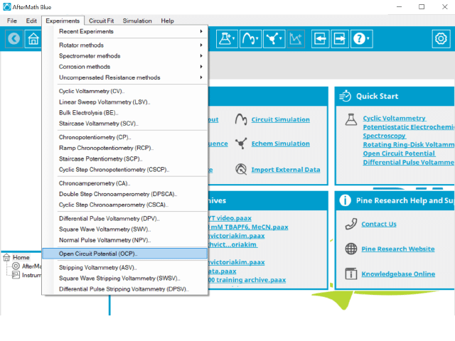
Figure 1. Open Circuit Potential (OCP) Expeirment Menu Selection in AfterMath

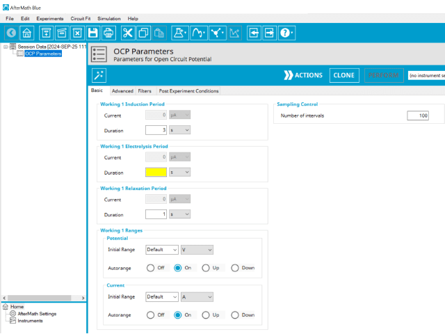
Doing so creates an entry within the archive, called OCP Parameters. In the right pane of the AfterMath application, several tabs will be shown (see Figure 2).

Figure 2. Open Circuit Potential (OCP) Experiment in AfterMath

As with most Aftermath methods, the experiment sequence is

Induction Period → Electrolysis Period → Relaxation Period → Post-Experiment Idle Conditions

Unlike most experiments, the Induction and Relaxation Periods are on the Basic Tab. The parameters for an OCP experiment are fairly simple compared to other methods in AfterMath.

In general, enter minimum required parameters on the Basic tab and press "Perform" to run an experiment. AfterMath will perform a quick audit of the parameters you entered to ensure their validity and appropriateness for the chosen instrument, followed by the initiation of the experiment. In some cases, users may desire to adjust additional settings such as filters, post- experiment conditions, and post-experiment processing before clicking the "Perform" button. Continue reading for detailed information about the fields on each unique tab.

3.1Basic Tab

TIP: Click the "I Feel Lucky" button on the top bar in AfterMath to automatically fill all required parameters with reasonable starting values. While the values provided may not be appropriate for your specific system, they are reasonable parameters with which to start your experiment, especially if you are new to the method.

The basic tab contains fields for the fundamental parameters necessary to perform an OCP experiment. AfterMath shades fields with
yellow when a required entry is blank and shades fields pink when the entry is invalid (see Figure 3).

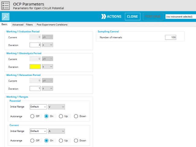
Open Circuit Potential Expeirment Basic Tab in AfterMath

Figure 3. Open Circuit Potential (OCP) Basic Tab in AfterMath

During the induction period, a set of initial conditions are applied to the electrochemical cell and the cell equilibrates at these conditions. Data are not collected during the induction period, nor are they shown on the plot during this period. For this method, current = 0 and as such, AfterMath will show an induction current field that is grayed out.

After the induction period, the potential difference is recorded when there is no current, which is called the electrolysis period. For this method, current = 0 and as such, AfterMath will show an electrolysis current field that is grayed out. The potentiostat ensures no current enters the system while simultaneously measuring the potential vs. REF. During the electrolysis period, the potential is recorded at regular intervals as specified on the Basic tab. Sampling control defines the number of intervals (number of data points) collected during the electrolysis period. With Electrolysis period duration, a sampling rate can be defined as,

$\displaystyle {\textrm{sampling rate}=\frac{\textrm{number of intervals}}{\textrm{electrolysis period duration}}}$

Users should enter a number of intervals that their analysis requires. Commonly, OCP experiments are sampled at a lower rate (1 sample/s). Not all sampling rates are allowed due to differences in hardware (WaveNow series vs. WaveDriver series, for example).

NOTE: Not all sampling rates are possible. When users enter a number of intervals that is not allowed, AfterMath will prompt the user with an "Interval too short" error. Change the number of intervals and try again. In general, integer values at moderate rates are most often possible.

The Electrode Range group contains the initial current and potential range fields. These field settings within the Electrode Range group explicitly define the initial current and/or potential ranges used by the potentiostat during the experiment. Additionally, a field for Autorange control for both potential and current appear on this tab. Autorange employs algorithms to adjust the current and potential ranges, as needed, to the most appropriate ranges available to match the measured signal(s). More information on autorange is available elsewhere on the knowledgebase.

The experiment concludes with a relaxation period. During the relaxation period, a set of final conditions (specified on the Advanced tab) are applied to the electrochemical cell and the cell equilibrates at these conditions. Data are not collected during the induction period, nor are they shown on the plot during this period. For this method, current = 0 and as such, AfterMath will show a relaxation current field that is grayed out.

A plot of the typical experiment sequence, containing labels of the fields on the Basic tab, helps to illustrate the sequence of events in a BE experiment (see Table 1 and Figure 4). Again, given that different electrode modes are possible, the illustrations provided here assume controlled potential (POT) mode; however, other modes such as controlled current (GAL) are analogous to these figures, with different units on the y-axis.

The table below lists the group and field names and symbol for each parameter associated with this experiment (see Table 1).

Group Name	Field Name	Symbol
Induction Period	Current	$I_{IND}=0$
Induction Period	Duration	$T_{IND}$
Electrolysis Period	Current	$I_{E}=0$
Electrolysis Period	Duration	$T_{E}$
Relaxation Period	Current	$I_{RLX}=0$
Relaxation Period	Duration	$T_{RLX}$
Sampling Control	Number of Intervals	$N_{INT}$

Table 1. Basic Tab Group Names, Field Names, and Symbols.

Open Circuit Potential (OCP) Experiment Basic Tab in AfterMath

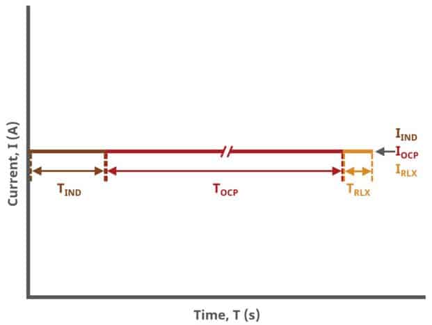
Figure 3. Open Circuit Potential (OCP) Basic Tab Field Diagram

At the end of the relaxation period, the post-experiment idle conditions are applied to the cell, and the instrument returns to the idle state. The default plot generated from this experiment is a plot of potential vs. time.

3.2Advanced Tab

The OCP Advanced tab contains two groups for iR Compensation and for Experiment End Trigger (see Figure 5).

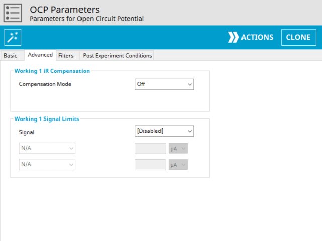
Figure 5. Open Circuit Potential (OCP) Experiment Advanced Tab

Detailed description of the iR Compensation Mode is provided elsewhere on the knowledgebase. This mode is used to correct for uncompensated resistance in the electrochemical cell.

In an OCP experiment, the researcher may want to have AfterMath monitor the response and then stop the experiment at a specific potential. This value is called a trigger and is set in the Experiment End Trigger group on the Advanced tab (see Figure 5). For OCP, the only trigger signal available is potential. Once this potential limit is reached (as defined), the OCP experiment terminates and retains the data collected up to the trigger endpoint.

3.3Filters and Post Experiment Conditions Tab

The Filters tab provides access to potentiostat hardware filters, including stability, excitation, current response, and potential response filters. Pine Research recommends that users contact us for help in making changes to hardware filters. Advanced users may have an easier time changing the automatic settings on this tab. Filter settings fields are shown for WK1 (working electrode #1) as well as for WK2 (working electrode #2) regardless of the potentiostat connected to AfterMath.

By default, the potentiostat disconnects from the electrochemical cell at the end of an experiment. There are other options available for what these post-experiment conditions can be and are controlled by setting options on the Post Experiment Conditions tab.

4Sample Experiment

As described, OCP is a fairly basic (and boring) experiment. Here, 2 mM of K₃Fe(CN)₆ in 0.1 M KCl at a 2 mm OD Pt WKG, Pt mesh CE, and Ag/AgCl RE was used to measure OCP. When $i=0$ the system measured a constant OCP of about +487.5 mV vs. REF.

OCP Expeirment with Potassium Ferricyanide Solution

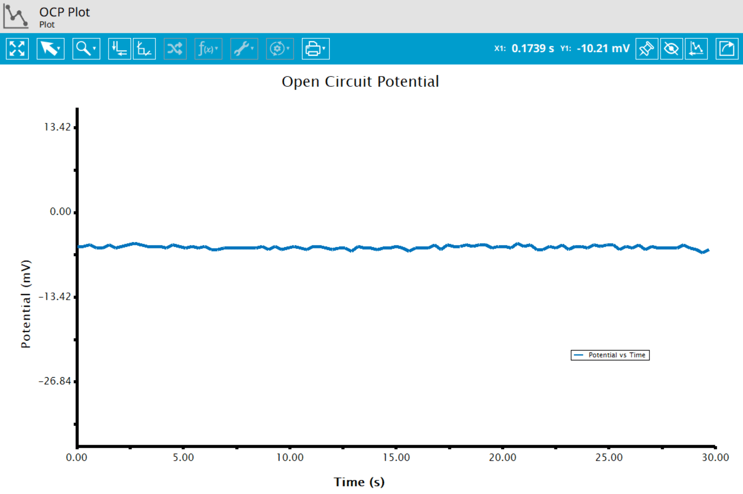
Figure 6. OCP Experiment with Potassium Ferricyanide Solution

5Example Applications

Examples of OCP are not entirely interesting, as it is mostly used as a tool for other advanced methods. The relatively simple nature of this technique does not have the typical example cases that other methods provide. Here, we provide a simple example from sample data. For the common electrochemical couple ferricyanide,

$\displaystyle K_3Fe(CN)_6 +e\rightleftharpoons K_4Fe(CN)_6 \hspace{10em} E^0=0.230 V$

During an OCP measurement, a stable potential of 0.275 V vs. REF was measured for 3 minutes at 25°C. With these data, we can use the Nernst equation to find the approximate conentration ratio of $O$ and $R$ ,

$\displaystyle E = E^{0'} + \frac{RT}{nF} \ln {\left(\frac{[K_3Fe(CN)_6]}{[K_4Fe(CN)_6]}\right)}$

The ratio of oxidized to reduced species can then be calculated (using the Nernst Equation)

$\displaystyle 0.275 \: V=0.230 \: V+0.0257 \: V\ln{\left(\frac{[K_3Fe(CN)_6]}{[K_4Fe(CN)_6]}\right)}$
$\displaystyle \vdots$
$\displaystyle 5.76=\frac{[O]}{[R]}$

The ratio of K₃Fe(CN)₆ to K₄Fe(CN)₆ in this example is 5.76:1; therefore, the solution contains approximately 85% K₃Fe(CN)₆ and 15% K₄Fe(CN)₆at the time OCP was measured.

How can we help? What do you want to learn? Search our knowledgebase.

Basic Methods

Open Circuit Potential (OCP)

ARTICLE TAGS

RELATED PRODUCTS

Article Contents/Section Navigation

1Technique Overview

2Fundamental Equations

3Experimental Setup in AfterMath

3.1Basic Tab

3.2Advanced Tab

3.3Filters and Post Experiment Conditions Tab

4Sample Experiment

5Example Applications

6References

Questions? Find Answers.

Software

Applications

Theory

Product Specifications