Differential Pulse Voltammetry (DPV)

Last Updated: 1/5/23 by Alex Peroff

ARTICLE TAGS

AfterMath DPV,
differential pulse voltammetry,
DPV,
current vs. potential

Capable Potentiostats

AFTERMATH LINKS

Article Contents/Section Navigation

1Technique Overview

Differential Pulse Voltammetry (DPV) is a potentiostatic method that offers some advantages to common techniques like Cyclic Voltammetry (CV), in that the waveform is a series of pulses increasing along a linear baseline. The way in which the current is measured at each pulse aids in minimizing the measurement of background (charging) current. Related pulse-type methods include Normal Pulse Voltammetry (NPV) and Square Wave Voltammetry (SWV).

Differential Pulse Voltammetry (DPV) is a pulse technique that is designed to minimize background charging currents. The waveform in DPV is a sequence of pulses where a baseline potential is held for a specified period of time prior to the application of a potential pulse. Current is sampled, at time ${\tau}'$ , just prior to the application of the potential pulse. The potential is then stepped by a small amount (typically 100 mV) and current is sampled again, at time $\tau$ at the end of the pulse. The potential of the working electrode is then stepped back by a lesser value than during the forward pulse such that baseline potential of each pulse is incremented throughout the sequence.

As with many other methods, users can initially sweep positively (towards an anodic limit) or negatively (toward a cathodic limit) initially. Below, typical DPV waveforms are shown for illustration, using only an increasing positive pulse sequence.

INFO: Initial sweep direction can be positive-increasing or negative increasing. Not all possibilities have been provided as examples in this article. Users must tailor their parameters to suit their specific electrochemistry. Contact us with any questions or additional assistance.

In the simplest case, when Segments (S_N) = 1 (see Figure 1), potential pulses step along a linear baseline from an initial to final potential, sampling current at specified intervals (see Figure 2).

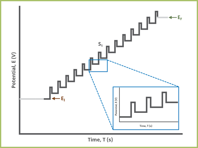
Figure 1. Differential Pulse Voltammetry (DPV) One Segment Waveform

Current is sampled, at time ${\tau}'$ (T_{DP, PRE}), just prior to the application of the potential pulse. The potential is then stepped by a small amount (typically 100 mV) and current is sampled again, at time $\tau$ (T_{DP, POST}) at the end of the pulse (see Figure 7). These sampling periods are selected to allow sufficient time for non-Faradaic (charging) current to decay such that primarily only current arising from Faradaic reactions is reported. The difference in current at these two periods for each pulse is plotted against potential results in a differential voltammogram, as

$\delta i=i(\tau)-i(\tau')$

In a later Section (Experimental Setup in AfterMath - Basic Tab), the pulse parameters are defined in detail (see Table 1 and Figure 7).

When Segments (S_N) = 2 (see Figure 2), potential pulses step along a linear baseline from an initial potential to vertex potential and then to final potential, sampling current at specified intervals. Again, the current is sampled in the same fashion as DPV experiments with other Segment values (see Figure 7).

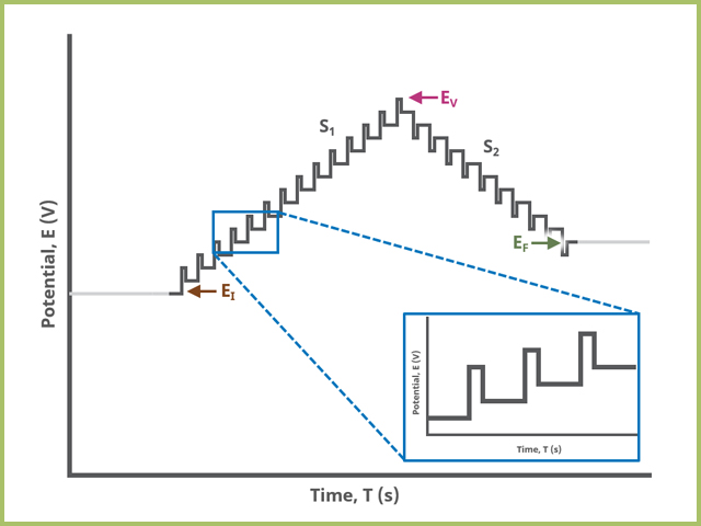
Differential Pulse Voltammetry (DPV) Two Segment Waveform

Square Figure 2. C

When Segments (S_N) = 3 (see Figure 3), potential pulses step along a linear baseline from an initial potential to upper potential to lower potential and then to final potential, sampling current at specified intervals. Again, the current is sampled in the same fashion as DPV experiments with other Segment values (see Figure 7).

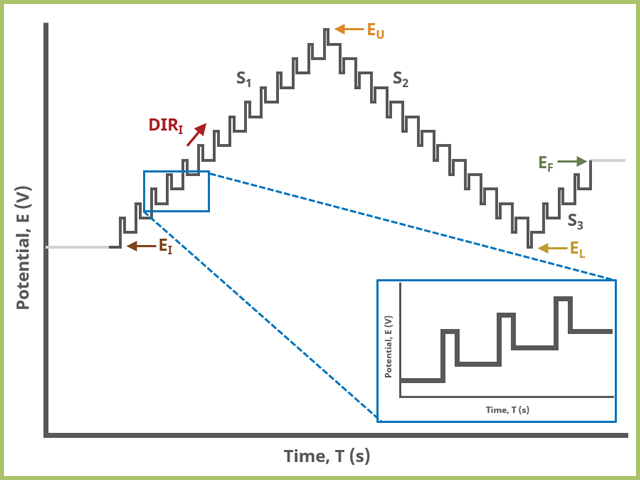
Figure 3. Differential Pulse Voltammetry (DPV) Three Segment Waveform

2Fundamental Equations

The following is a brief introduction to the theory of DPV. Please see Bard and Faulkner for a more complete description. For additional information on the cyclic form of DPV, consult the paper by Drake et al.

Consider the reaction,

$O + e^- \rightarrow R$

where $O$ is reduced in a one electron step to $R$ . At values sufficiently more positive than $E^{0'}$ no faradaic current flows before the potential step (to more negative values). The application of the potential step does not produce an appreciable increase in current; thus, the differential is very small. At values significantly negative of $E^{0'}$ the baseline potential is reducing $O$ at a maximum rate. The application of a small potential step (towards more negative values) is unlikely to increase the rate of reduction; thus, the differential current is again small. Only at potentials around $E^{0'}$ will the differential current be significant. The period during the application of the baseline potential has $O$ being reduced at some rate. The potential step (to more negative values) increases the rate of reduction and hence the differential current will be significant. Under normal conditions (pulse height < 100 mV) the height of the peak can is given by the equation

$\displaystyle({\delta}t)_{max} = \frac{nFAD_O^{1/2}C_O^*}{{\pi}^{1/2}({\tau}-{\tau}')} \left({\frac{1-\sigma}{1+\sigma}}\right)$

where $n$ is the number of electrons, $F$ is Faraday's Constant (96485 C/mol), $A$ is the electrode area (in cm²), $D$ is the diffusion coefficient (in cm²/s), $C_O^*$ is the concentration of electroactive species (in mol/cm³) and $\sigma$ is given by

$\displaystyle\sigma = \left(\frac{nF}{RF}\frac{{\Delta}E}{2}\right)$

where ${\Delta}E$ is the pulse height, $T$ is the temperature ( $K$ ) and $R$ is the Universal Gas Constant (8.314 J/mol⋅K).

As mentioned in the Advanced parameters tab (discussed in a subsequent section), the direction of the pulse should not affect the results. Consider the same reaction above where $O$ is reduced in a one-electron step to $R$ . At values sufficiently more positive than $E^{0'}$ no faradaic current flows before the potential step (towards more positive values). The change in current due to the potential step is also insignificant enough to cause a Faradaic current; thus, the differential is very small. At values significantly negative of $E^{0'}$ the baseline potential is reducing $O$ at a maximum rate. The application of a small potential pulse (towards more positive values) does not decrease the rate of reduction and hence the differential current is again small. Only at potentials around $E^{0'}$ will the differential current be significant. The period during the application of the baseline potential has $O$ being reduced at some rate. The potential step (to more positive values) decreases the rate of reduction and hence the differential current will be significant; therefore, the direction of the potential step has no effect on the differential current observed.

3Experimental Setup in AfterMath

To perform a differential pulse voltammetry experiment in AfterMath, choose Differential Pulse Voltammetry (DPV) from the Experiments menu (see Figure 4).

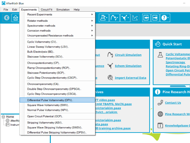
Figure 4. Differential Pulse Voltammetry (DPV) Experiment Menu Selection in AfterMath

Doing so creates an entry within the archive, called DPV Parameters. In the right pane of the AfterMath application, several tabs will be shown (see Figure 5).

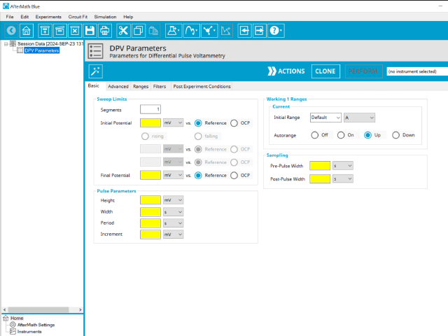
Figure 5. Differential Pulse Voltammetry (DPV) Experiment Basic Tab

As with most Aftermath methods, the experiment sequence is

Induction Period → Pulse Sequence → Relaxation Period → Post-Experiment Idle Conditions

Continue reading for detailed information about the fields on each unique tab.

3.1Basic Tab

TIP: Click the AutoFill button ("I Feel Lucky" prior to May 2019) on the top bar in AfterMath to automatically fill all required parameters with reasonable starting values. While the values provided may not be appropriate for your specific system, they are reasonable parameters with which to start your experiment, especially if you are new to the method.

The basic tab contains fields for the fundamental parameters necessary to perform a DPV experiment. AfterMath shades fields with yellow when a required entry is blank and shades fields pink when the entry is invalid (see Figure 6).

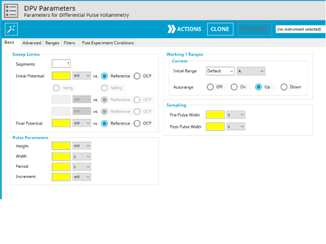
Normal Pulse Voltammetry (NPV) Basic tab in AfterMath

Figure 6. Differential Pulse Voltammetry (DPV) Basic tab in AfterMath

During the induction period, a set of initial conditions are applied to the electrochemical cell and the cell equilibrates at these conditions. Data are not collected during the induction period, nor are they shown on the plot during this period. Users will define induction period parameters on the Advanced Tab.

After the induction period, the potential of the working electrode is stepped through a series of increasing pulses from the Initial potential to the Final potential. The potential is incremented with each successive pulse according to the Pulse increment. Current is measured at the time obtained by subtracting the Pulse sampling width window from the Pulse width. In a typical experiment, Segments = 1 and there is a single series of pulses moving along the linear baseline from initial to final potential. Some may want to reverse the pulses (move in the opposite direction), accomplished by adjusting the number of segments to be > 1. By adjusting the number of segments, users can create variants of the DPV technique. Cyclic Differential Pulse Voltammetry consists of cycling (through a series of potential pulses also) the potential of the working electrode between an Upper potential and a Lower potential (Segments = 2 or 3).

The parameter settings for pulse-type experiments are often not as clear as with something more simple like Cyclic Voltammetry (a sweep method ). Refer to Figure 7 below when understanding each parameter of the DPV pulse. Further, clicking "AutoFill" ("I Feel Lucky" in older versions of AfterMath) provides reasonable starting parameters if you are unsure of typical values used in these experiments. Most often, research journal articles describe the DPV pulse sequence used, which can be replicated using AfterMath.

The experiment concludes with a relaxation period. During the relaxation period, a set of final conditions (specified on the Advanced tab) are applied to the electrochemical cell and the cell equilibrates at these conditions (set on the Advanced Tab). Data are not collected during the induction period, nor are they shown on the plot during this period.

At the end of the relaxation period, the post-experiment idle conditions are applied to the cell and the instrument returns to the idle state.

A plot of the typical experiment sequence, containing labels of the fields on the Basic tab, helps to illustrate the sequence of events in a DPV experiment (see Table 1 and Figure 7).

The table below lists the group and field names and symbols for each parameter associated with this experiment (see Table 1).

Group Name	Field Name	Symbol
Sweep (Sweep limits)	Segments	$S_N$
Sweep (Sweep limits)	Initial Potential	$E_I$
Sweep (Sweep limits)	Initial Direction	$DIR_I$
Sweep (Sweep limits)	Upper Potential	$E_U$
Sweep (Sweep limits)	Vertex Potential	$E_V$
Sweep (Sweep limits)	Lower Potential	$E_{LOW}$
Sweep (Sweep limits)	Final Potential	$E_F$
Differential Pulse (Pulse parameters)	Height	$E_{DP, \;H}$
Differential Pulse (Pulse parameters)	Width	$T_{DP, \;W}$
Differential Pulse (Pulse parameters)	Period	$T_{DP, \;P}$
Differential Pulse (Pulse parameters)	Increment	$E_{DP, \;I}$
Differential Pulse (Sampling)	Pre-Pulse width	$T_{DP, \;PRE} \;(\tau ')$
Differential Pulse (Sampling)	Post-pulse width	$T_{DP, \;POST} \; (\tau)$

Table 1. Basic Tab Group Names, Field Names, and Symbols.

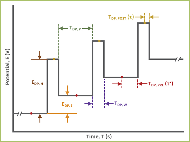
Figure 7. Differential Pulse Voltammetry (DPV) Pulse Sequence Detail

3.2Advanced Tab

The DPV Advanced tab contains groups for Induction Period, Relaxation Period, Pulse options, and iR Compensation (see Figure 8).

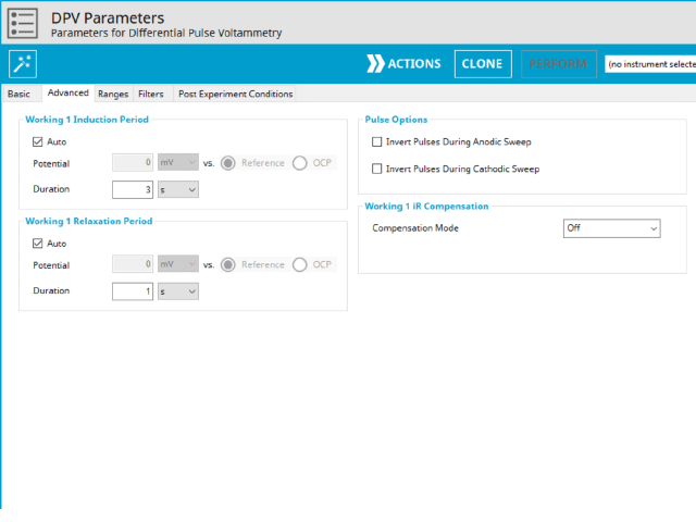
Figure 8. Differential Pulse Voltammetry (DPV) Experiment Advanced Tab in AfterMath

Induction Period is the first step in a DPV experiment if the Duration is >0 s. During the induction period, the specified current is applied to the cell for the specified duration. During this period, data are not collected. The Induction Period is believed to "calm" the cell prior to intentional perturbation. More on Induction Period is found within the knowledgebase.

Relaxation Period is the last step in a DPV experiment if the Duration is >0 s. During the relaxation period, the specified current is applied to the cell for the specified duration. During this period, data are not collected. The Relaxation Period is believed to "calm" the cell after intentional perturbation. More on Relaxation Period is found within the knowledgebase.

A unique set of options for DPV is the ability to invert the pulse direction. Within the "Pulse" options are two checkbox options to invert pulses during the anodic sweep and to invert the pulses during the cathodic sweep. The directionality of a DPV is determined by selection of initial, vertex, upper, lower, and final potential, dependent on the Number of Segments (S_N). When the pulse sequence moves in the direction of increasing positive potential, this is the anodic sweep. Conversely, when the pulse sequence moves in the direction of increasing negative potential, this is the cathodic sweep. To better understand and visualize these pulse options, a figure with each set of conditions has been prepared (see Figure 9).

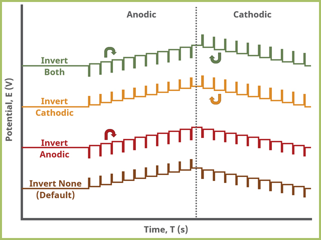
Figure 9. Differential Pulse (DPV) Pulse Inversion Options

Lastly, the iR Compensation group allows users to adjust the cell feedback to accommodate a known resistive drop between working and reference electrodes. Not all potentiostats from Pine Research support iR compensation. The WaveDriver series support iR compensation by positive feedback and current interrupt. The WaveDriver 100, WaveDriver 200, and WaveDriver 40 support EIS-based iR compensation. The WaveNow series (including the WaveNano and WaveNow^XV WaveNowXV Potentiostat/Galvanostat Basic Bundle ) and the CBP bipotentiostat do not support iR compensation of any type. More information about iR compensation, including understanding how it works and how to determine the resistance, consult the knowledgebase article on the topic.

The general experimental flow for a DPV experiment is provided below (see Figure 10), highlighting the Induction period, DPV Pulse Sequence, and Relaxation period. Following the relaxation period, the post-experiment conditions are applied.

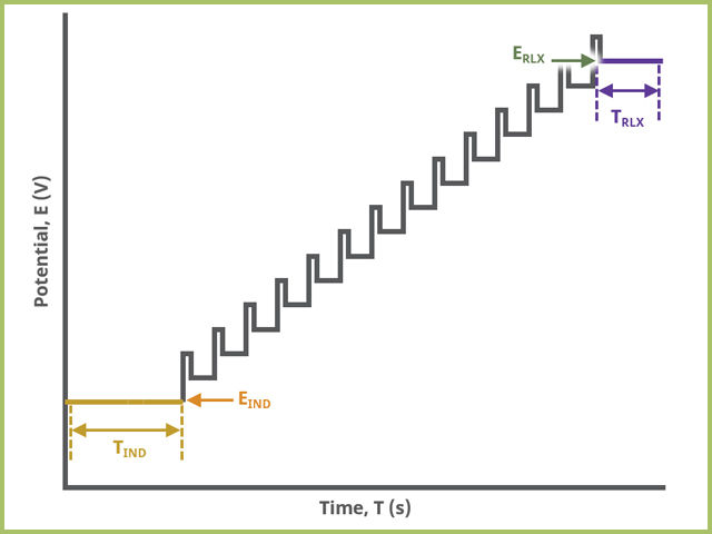
Figure 10. Differential Pulse Voltammetry (DPV) Experiment Sequence in AfterMath

3.3Ranges, Filters, and Post Experiment Conditions Tab

In nearly all cases, the groups of fields on the Ranges tab are already present on the Basic tab. The Ranges tab shows an Electrode Range group and depending on the experiment shows either, or both, current and potential ranges and the ability to select an autorange function. The fields on this tab are linked to the same fields on the Basic tab (for most experiments). Changing the values on either the Ranges tab or on the Basic tab changes the other set. In other words, the values selected for these fields will always be the same on the Ranges tab and on the Basic tab. More on ranges is found within the knowledgebase, as is for autorange.

The Filters tab provides access to potentiostat hardware filters, including stability, excitation, current response, and potential response filters. Pine Research recommends that users contact us for help in making changes to hardware filters. Advanced users may have an easier time changing the automatic settings on this tab. Filter settings fields are shown for WK1 (working electrode #1) as well as for WK2 (working electrode #2) regardless of the potentiostat connected to AfterMath.

By default, the potentiostat disconnects from the electrochemical cell at the end of an experiment. There are other options available for what these post-experiment conditions can be and are controlled by setting options on the Post Experiment Conditions tab.

4Sample Experiment

Below are the typical results for DPV for the oxidation of a 1.4 mM solution of K₄Fe(CN)₆ in 0.1 M phosphate buffer (see Figure 11). The specific parameters for this experiment are as follows:

pH = 6.8
3 mm glassy carbon WE
period = 100 ms
width = 10 ms
height = 50 mV
potential increment = 10 mV

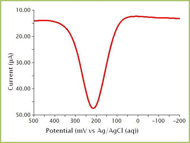
Figure 11. Differential Pulse Voltammogram of a Potassium Ferrocyanide Solution in Phosphate Buffer

Below are the typical results for a two segment Cyclic Differential Pulse Voltammetry (CDPV) for the oxidation and reduction ofK₄Fe(CN)₆ in 0.1 M phosphate buffer (see Figure 12). Crosshair tools have been added to show that peak positions and peak heights should be identical in CDPV for a fully reversible system. The specific parameters for this expeirment are as follows:

pH = 6.8
3 mm glassy carbon WE
period = 100 ms
width = 10 ms
height = 50 mV
potential increment = 10 mV

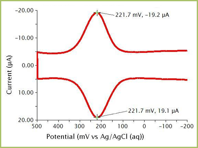
Figure 12. Cyclic Differential Pulse Voltammogram of a Potassium Ferrocyanide Solution in Phosphate Buffer

5Example Applications

The first example uses DPV to examine the pH dependence of redox potential for an electron and proton transfers in tryptophan and tyrosine. Sjödin et al. used the pH dependence of the redox potential to calculate ${\Delta} G$ values for different reaction pathways and thus determine that the mechanism can be a one-step or two steps depending on several factors.

In another example, Miles and Murray use DPV to examine the quantized double layer charging of hexanethiolate-coated monolayer-protected Au₁₄₀ clusters (AuMPCs). They used DPV to resolve 13 individual peaks related to AuMPC core charging over a 3 V window in CH₂Cl₂ at lowered temperatures. Though peaks are visible using CV, DPV provides the necessary resolving power, by suppressing background currents, to separate out all 13 peaks.

How can we help? What do you want to learn? Search our knowledgebase.

Voltammetric Methods

Differential Pulse Voltammetry (DPV)

ARTICLE TAGS

Capable Potentiostats

RELATED PAGES

AFTERMATH LINKS

Article Contents/Section Navigation

1Technique Overview

2Fundamental Equations

3Experimental Setup in AfterMath

3.1Basic Tab

3.2Advanced Tab

3.3Ranges, Filters, and Post Experiment Conditions Tab

4Sample Experiment

5Example Applications

6References

Questions? Find Answers.

Software

Applications

Theory

Product Specifications