1. Plotting Conventions - Nyquist Plot
There are two standard types of plots generated from five-column EIS data: Nyquist and Bode plots. A Nyquist plot normally consists of  vs.
vs.  , and this type of plot is most commonly used to identify distinctive patterns and shapes in the data (see Figure 1 for examples of Nyquist plots for several different circuit networks).
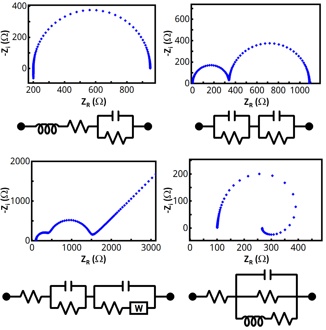
Figure 1: Example Nyquist Plots for Different Circuit Networks
The imaginary impedance values on a Nyquist plot are commonly inverted, or conversely the axis is sometimes displayed in reverse numerical order, due to the fact that almost all values are normally less than zero and it is more convenient to view shapes and patterns primarily in the first quadrant on a Cartesian graph (see Figure 1).
Another convention traditionally applied to Nyquist plots is orthonormality, also sometimes called orthogonality, which refers to the usage of a 1:1 ratio for the visual scale of x- and y-axes. Note that this does not necessarily mean the numerical scales of the axes need necessarily be identical (see plots in Figure 1 for example). One simple way to think of this principle is that when drawing lines on an orthonormal plot around identical values on both axes, it would always make a perfect square (e.g., connect the points (0,0), (0,100), (100,100), and (100,0), and it will be a perfect square).
Historically, orthonormality was used exclusively on Nyquist plots because some of the ubiquitous shapes (e.g., semicircles and tilted lines) are more easily discerned when viewed on an orthonormal plot. In modern times, however, some of this plotting necessity has become diminished with the advent of circuit fitting software. While non-idealities in data can be observed through distorted semicircles and tilted line angles on an orthonormal Nyquist plot, they are also easily visualized and quantified via circuit fitting algorithms. It can also occasionally be inconvenient to force orthonormality on some Nyquist plots if the data becomes concentrated to a small portion of the plot, leaving large swaths of empty graphical space (e.g., upper right plot on Figure 1).
Those points notwithstanding, it is still widely considered standard form to employ orthonormality to Nyquist plots, and most published EIS data use this convention. Therefore, it is generally recommended that the user prepare orthonormal Nyquist plots when presenting their EIS data.
2. Plotting Conventions - Bode Plots
The second standard type of plot used with EIS data is a Bode plot. A Bode plot is a double-axis plot consisting of both  vs.
vs.  (on the primary vertical axis) and
  vs. (on the secondary vertical axis). Frequency and impedance magnitude are normally plotted on a logarithmic scale, while the phase angle is displayed linearly (see Figure 2 for examples of Bode plots for several different circuit networks).
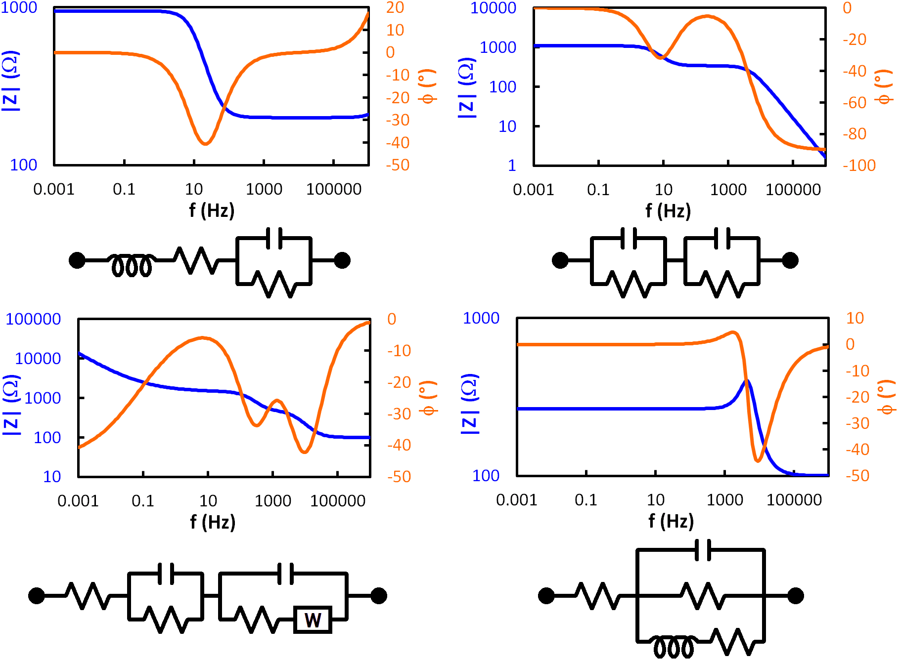
Figure 2: Example Bode Plots for Different Circuit Networks
Observing the phase angle on a Bode plot is a quick way to understand the type of circuit behavior a system is experiencing at any particular frequency. For example, a phase angle of 0° corresponds to an ideal resistor, +90° corresponds to an ideal inductor, and -90° corresponds to an ideal capacitor. Values in between may indicate mixed behavior or non-ideality depending on the system under study.
Bode plots also allow easy determination of frequency values, compared with Nyquist plots where frequency values are not plotted. Generally, the lower-leftmost points on a Nyquist plot correspond to the highest frequencies, and following the trace to the right moves from high to low frequency.
