
1. Technique Overview
Chronoamperometry (CA) is a widely used method in electrochemistry, due in part to its relative ease of implementation and analysis. CA is highly sensitive, as most electrochemical methods are; however, CA is poorly selective. In an unstirred cell, in response to a potential step perturbation, electrochemically active species will diffuse to the surface of the working electrode as a function of the potential applied. At the onset of a potential step, a large current arising from ion flux to the electrode surface to balance the change in potential gives rise to a capacitive current, which decays rapidly (just like any RC circuit). The concentration of electrochemically active species near the electrode surface decays with distance from the electrode and the arrival of species to the surface is diffusion limited; therefore, Faradaic current near the electrode surface decays over time as the mass transport limit is reached. These currents provide a typical exponential decay curve, which is described by the Cottrell equation.
2. Fundamental Equations
The following is a basic description of the theory behind Chronoamperometry. Please see the literature for a more detailed description of the technique1.
Consider the general reaction
 (1)
(1)with a formal potential 


When the current is diffusion-limited in CA, the current-time response is described by the Cottrell equation2
 (2)
(2)where 


3. Experimental Setup in AfterMath
To perform a chronoamperometry experiment in AfterMath, choose Chronoamperometry (CA) from the Experiments menu (see Figure 1).
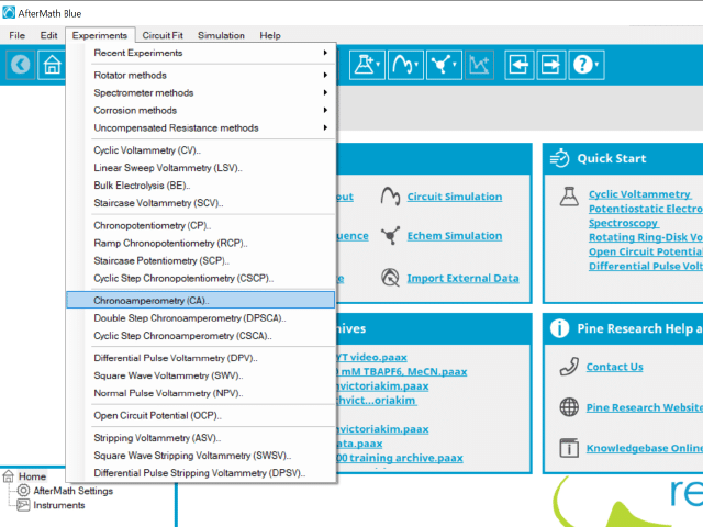
Figure 1: Chronoamperometry (CA) Experiment Menu Selection in AfterMath
Doing so creates an entry within the archive, called CA Parameters. In the right pane of the AfterMath application, several tabs will be shown (see Figure 2).
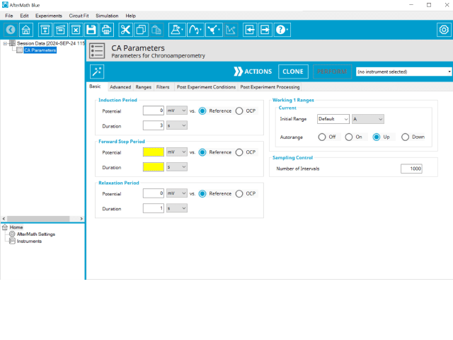
Figure 2: Chronoamperometry (CA) Experiment Basic Tab
As with most Aftermath methods, the experiment sequence is
Induction Period → Electrolysis Period (Forward Step Period) → Relaxation Period → Post-Experiment Idle Conditions
Unlike most experiments, the Induction and Relaxation Periods are on the Basic Tab. The parameters for a CA experiment are fairly simple compared to other methods in AfterMath.
In general, enter minimum required parameters on the Basic tab and press “Perform” to run an experiment. AfterMath will perform a quick audit of the parameters you entered to ensure their validity and appropriateness for the chosen instrument, followed by the initiation of the experiment. In some cases, users may desire to adjust additional settings such as filters, post- experiment conditions, and post-experiment processing before clicking the “Perform” button. Continue reading for detailed information about the fields on each unique tab.
3.1. Basic Tab
The basic tab contains fields for the fundamental parameters necessary to perform a CA experiment. AfterMath shades fields with
yellow when a required entry is blank and shades fields pink when the entry is invalid (see Figure 3).
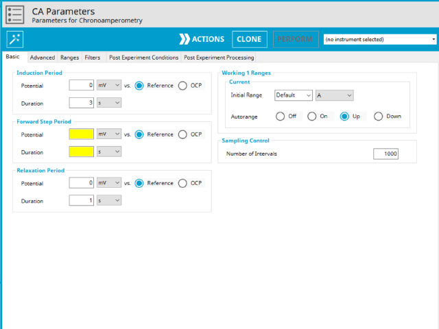
Figure 3: Chronoamperometry (CA) Basics Tab in AfterMath
During the induction period, a set of initial conditions are applied to the electrochemical cell and the cell equilibrates at these conditions. Data are not collected during the induction period, nor are they shown on the plot during this period.
After the induction period, the potential applied to the working electrode is stepped to the specified value for the duration of the experiment, which is called the electrolysis period (on CA, this group may be labeled Forward Step Period, depending on your version of AfterMath). The potentiostatic circuit of the instrument maintains constant applied potential relative to the reference electrode while simultaneously measuring the current at the working electrode. During the electrolysis period, potential and current at the working electrode are recorded at regular intervals as specified on the Basic tab. Sampling control defines the number of intervals (number of data points) collected during the electrolysis period. With Electrolysis period duration, a sampling rate can be defined as,

Users should enter a number of intervals that their analysis requires. Commonly, CA experiments are sampled at a lower rate (1 sample/s). Not all sampling rates are allowed due to differences in hardware (WaveNow series vs. WaveDriver series, for example).
The Electrode Range group contains the initial current and potential range fields. These field settings within the Electrode Range group explicitly define the initial current and/or potential ranges used by the potentiostat during the experiment. Additionally, a field for Autorange control for both potential and current appear on this tab. Autorange employs algorithms to adjust the current and potential ranges, as needed, to the most appropriate ranges available to match the measured signal(s). More information on autorange is available elsewhere on the knowledgebase.
The experiment concludes with a relaxation period. During the relaxation period, a set of final conditions (specified on the Advanced tab) are applied to the electrochemical cell and the cell equilibrates at these conditions. Data are not collected during the induction period, nor are they shown on the plot during this period.
A plot of the typical experiment sequence, containing labels of the fields on the Basic tab, helps to illustrate the sequence of events in a CA experiment (see Table 1 and Figure 4).


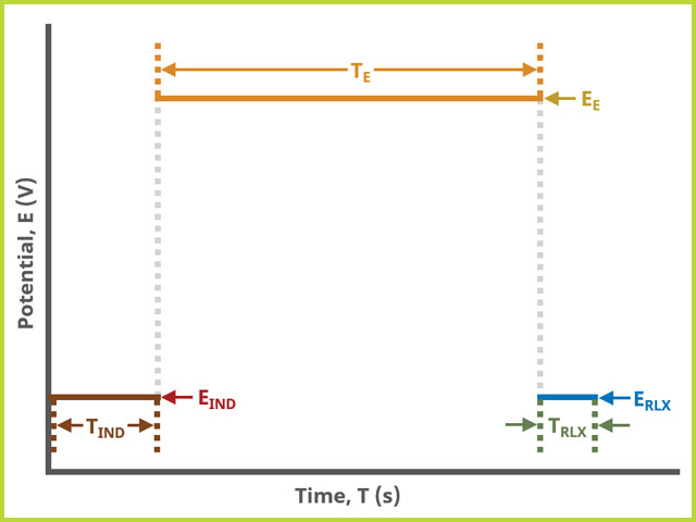
Figure 4: Chronoamperometry (CA) Basic Tab Field Diagram
At the end of the relaxation period, the post-experiment idle conditions are applied to the cell, the post-experiment processing tasks perform, and the instrument returns to the idle state. The default plot generated from the data is current vs. time.
3.2. Advanced Tab
The CA Advanced tab contains two groups for iR Compensation and for Experiment End Trigger (see Figure 5).
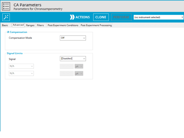
Figure 5: Chronoamperometry (CA) Advanced Tab
Detailed description of the iR Compensation Mode is provided elsewhere on the knowledgebase. This mode is used to correct for uncompensated resistance in the electrochemical cell.
In a CA experiment, the researcher may want to have AfterMath monitor the response and then stop the experiment at a specific current, potential, and/or charge. This value is called a trigger and is set in the Experiment End Trigger group on the Advanced tab (see Figure 5). For CA, the signals for the trigger can be potential, current, or charge.
3.3. Ranges, Filters, and Post Experiment Conditions Tab
In nearly all cases, the groups of fields on the Ranges tab are already present on the Basic tab. The Ranges tab shows an Electrode Range group and depending on the experiment shows either, or both, current and potential ranges and the ability to select an autorange function. The fields on this tab are linked to the same fields on the Basic tab (for most experiments). Changing the values on either the Ranges tab or on the Basic tab changes the other set. In other words, the values selected for these fields will always be the same on the Ranges tab and on the Basic tab. More on ranges is found within the support articles, as is for autorange.
The Filters tab provides access to potentiostat hardware filters, including stability, excitation, current response, and potential response filters. Pine Research recommends that users contact us for help in making changes to hardware filters. Advanced users may have an easier time changing the automatic settings on this tab.
By default, the potentiostat disconnects from the electrochemical cell at the end of an experiment. There are other options available for what these post-experiment conditions can be and are controlled by setting options on the Post Experiment Conditions tab.
3.4. Post-Experiment Processing Tab
At the completion of this experiment, there are additional post-processed plots that can optionally be generated. Additional plots will increase the size of the archive; however, if they are desired, it can save time to generate them automatically than manually later (see Figure 6).
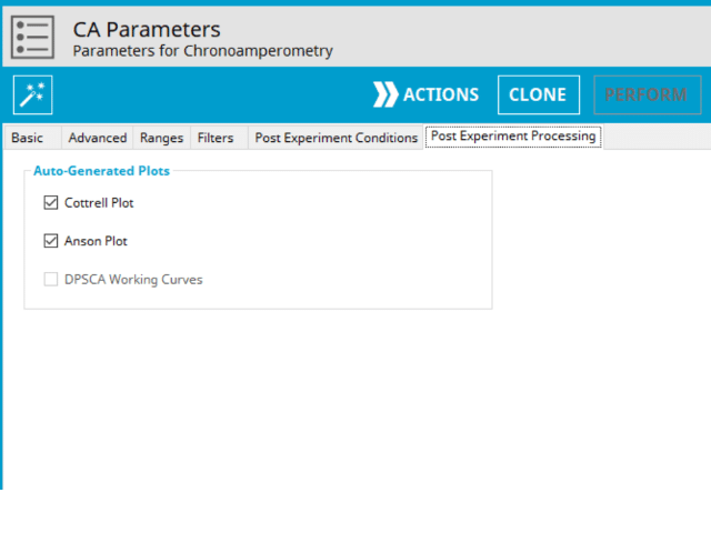
Figure 6: Chronoamperometry (CA) Post-Experiment Processing Tab
On the Post-Expeirment Processing Tab for CA, users can enable two additional plots: Cottrell Plot (see Figure 7) or Anson Plot (see Figure 8). Tick the checkbox next to the plot to add them to the archive following the completion of the experiment.
Ticking the box next to Cottrell Plot displays a plot of i vs. t-1/2 (see Figure 7). Ticking the box next to Anson Plot displays a plot of Q vs. t1/2 (see Figure 8). Note that for the Cottrell Plot, the level portion in the plot is actually the time prior to the current spike shown in the chronoamperogram (see Figure 8). That is, earlier time points are to the right in a Cottrell Plot. This is not the case for an Anson Plot because integrating the current with respect to time gives charge. The endpoint in an Anson Plot is the total amount of charge passed during the experiment. Monitoring the charge passed during an experiment is a variant of chronoamperometry called Chronocoulometry.
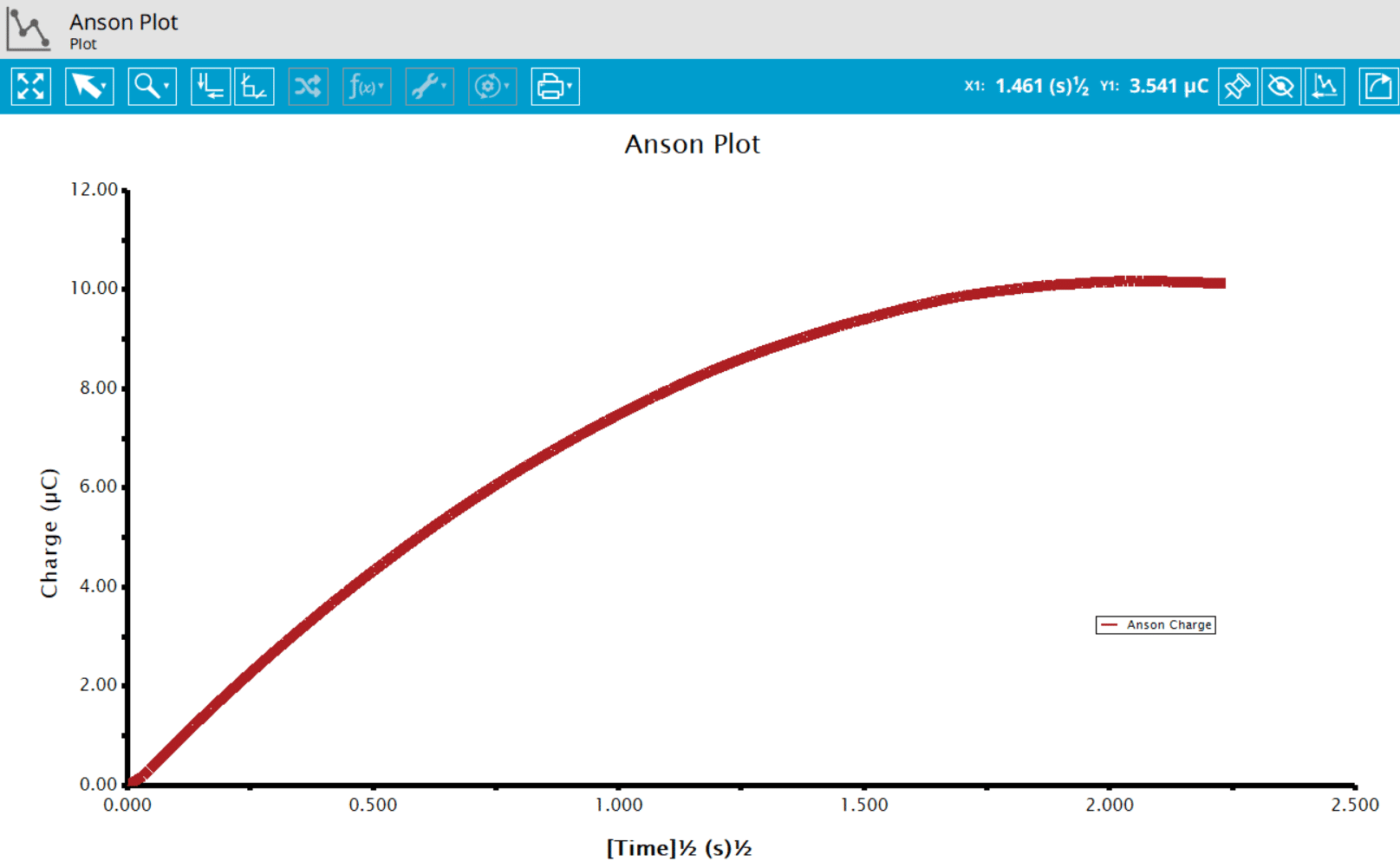
Figure 7: Chronocoulometric (Charge) Anson Plot of Acetominophen
4. Sample Experiment
The results for a 1 mM solution of acetominophen in aqueous saline solution are shown below (see Figure 9).
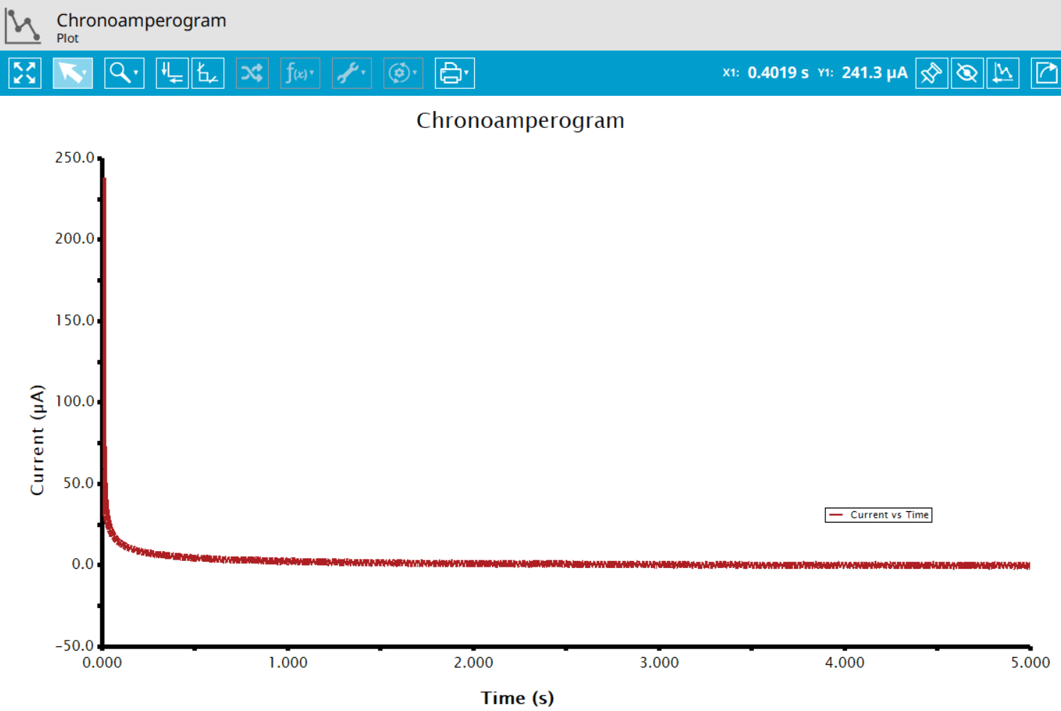
Figure 8: Sample Chronoamperogram of acetominophen at 800 mV vs Ag/AgCl
on a carbon screen printed electrode.
5. Example Applications
In the first example, Tennyson et. al used chronoampometry to determine the diffusion coefficients 

 (3)
(3)allows for the calculation of
In another example, researchers show how CA was used to measure extremely small diffusion coefficients of redox polyether hybrid cobalt bipyridine molten salts. Crooker and Murray performed chronoamperometry on a series of undiluted molten salts and were able to obtain diffusion coefficients as low as 10-17 cm2/s.4 The researchers obtained heterogeneous rate constants 
Here, chronoamperometry to directly measure rate constants. Smalley et al.5 examined a series of monolayers terminated with either a ferrocene or ruthenium redox moiety. For monolayers containing more than 11 methylene units, chronoamperometry was used to determine the heterogeneous rate constants 
In a modified CA experiment, researchers used chronocoulometry (CC, a post-experiment calculation of CA data). Wolfe et al. prepared a series of ferrocenated hexanethiolate protected Au nanoparticles6. Normally, thermogravimetric analysis (TGA) would be used to calculate the number of thiolates per nanoparticle; however, in this case, TGA was inconclusive due to a slow loss of mass over the applied temperature range. The researchers instead monitored the charge passed (Q) over time for the solution of nanoparticles of known concentration. By knowing the total charge passed and the particle concentration, they determined the number of ligands per nanoparticle. This is an excellent example of how electrochemistry can be used in place of more traditional characterization techniques.
In another example of using post-processed CA data, researchers employed chronocoulometry (CC, a post-experiment calculation of CA data), but rather than using it for quantification purposes, the researchers use it to evoke a change in the system. Zhang et al. use chronocoulometry with predefined endpoints to produce Ag nanoparticles of various shpaes and sizes that were confined to an electrode surface7. By varying the amount of charge passed the researchers were able to show that triangular nanoparticles oxidize first on the bottom edge, followed by triangular tips, followed by out-of-plane height. Since the researchers also coupled spectroscopy to their electrochemical experiments they were also able to show how the SPR band changes with nanoparticle shape evolution. This example illustrates how electrochemistry can be used to evoke a change in a system rather than simply used as a method to monitor changes or determine the physical parameters of the system.
6. Related Video
The following YouTube video provides a short introduction to chronoamperometry, and can be found along with other useful content on the Pine Research YouTube channel.
7. References
- Bard, A. J.; Faulkner, L. A. Electrochemical Methods: Fundamentals and Applications, 2nd ed. Wiley-Interscience: New York, 2000.
- Cottrell, F. G. Residual current in galvanic polarization regarded as a diffusiona problem. Z. Phys. Chem., 1903, 42, 385–431.
- Tennyson, A. G.; Khramov, D. M.; Varnado, C. D.; Creswell, P. T.; Kamplain, J. W.; Lynch, V. M.; Bielawski, C. W. Indirectly Connected Bis(N-Heterocyclic Carbene) Bimetallic Complexes: Dependence of Metal−Metal Electronic Coupling on Linker Geometry. Organometallics, 2009, 28(17), 5142-5147.
- Crooker, J. C.; Murray, R. W. Probing the Limits: Ultraslow Diffusion and Heterogeneous Electron Transfers in Redox Polyether Hybrid Cobalt Bipyridine Molten Salts. Anal. Chem., 2000, 72(14), 3245-3252.
- Smalley, J. F.; Finklea, H. O.; Chidsey, C. E. D.; Linford, M. R.; Creager, S. E.; Ferraris, J. P.; Chalfant, K.; Zawodzinsk, T.; Feldberg, S. W.; Newton, M. D. Heterogeneous Electron-Transfer Kinetics for Ruthenium and Ferrocene Redox Moieties through Alkanethiol Monolayers on Gold. J. Am. Chem. Soc., 2003, 125(7), 2004-2013.
- Wolfe, R. L.; Balasubramanian, R.; Tracy, J. B.; Murray, R. W. Fully Ferrocenated Hexanethiolate Monolayer-Protected Gold Clusters. Langmuir, 2007, 23(4), 2247-2254.
- Zhang, X.; Hicks, E. M.; Zhao, J.; Schatz, G. C.; Van Duyne, R. P. Electrochemical Tuning of Silver Nanoparticles Fabricated by Nanosphere Lithography. Nano Lett., 2005, 5(7), 1503-1507.