
1. Technique Overview
Chronopotentiometry (CP) is a galvanostatic method in which the current at the working electrode is held at a constant level for a given period of time. The working electrode potential and current are recorded as a function of time. Researchers employ this method to study chemical reaction mechanisms and kinetics. It is also frequently used to study batteries and electrodeposition. CP is typically performed in an unstirred electrochemical cell; although, some researchers employ rotating electrodes in conjunction with CP.
Typically, current is held constant between working and counter electrodes while potential is measured at the working electrode, relative to the reference electrode. Redox-active species diffuse to the working electrode surface to balance the applied current, until the diffusion-limited concentration of redox species reaches zero at the electrode surface, at which time potential changes to the redox potential of the next species, if present, in solution (which could be solvent). CP is also commonly used during battery charge and discharge experiments.
2. Fundamental Equations
Numerous texts thoroughly explain electrochemical theory and should be consulted for a complete understanding of this method1-3.
Consider the general reaction
 (1)
(1)with formal potential 


 (2)
(2)where 


For rapid electrode kinetics, the time-based Nernstian equation is
 (3)
(3)where 
 (4)
(4)A plot of 


3. Experimental Setup in AfterMath
To perform a chronopotentiometry experiment in AfterMath, choose Chronopotentiometry (CP) from the Experiments menu (see Figure 1).
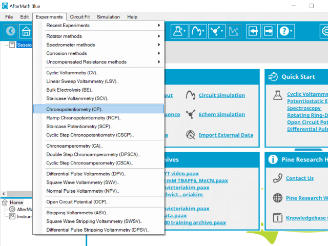
Figure 1: Chronopotentiometry (CP) Experiment Menu Selection in AfterMath
Doing so creates an entry within the archive, called CP Parameters. In the right pane of the AfterMath application, several tabs will be shown (see Figure 2).
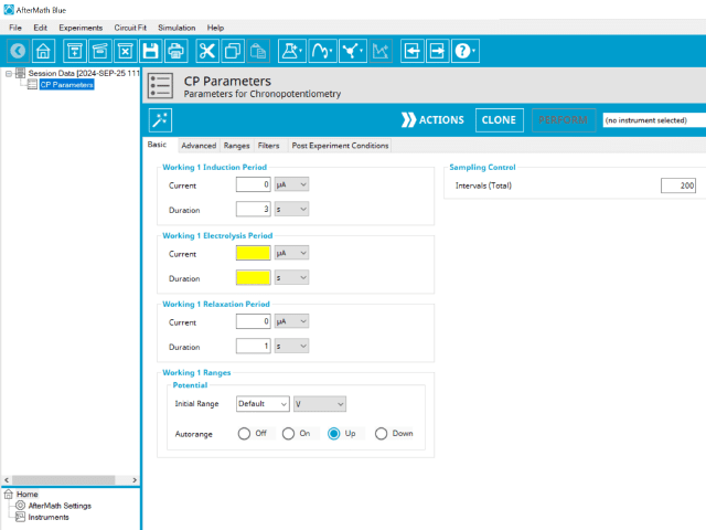
Figure 2: Chronopotentiometry (CP) Experiment in AfterMath
As with most Aftermath methods, the experiment sequence is
Induction Period → Electrolysis Period → Relaxation Period → Post-Experiment Idle Conditions
Unlike most experiments, the Induction and Relaxation Periods are on the Basic Tab. The parameters for a CP experiment are fairly simple compared to other methods in AfterMath.
3.1. Basic Tab
The basic tab contains fields for the fundamental parameters necessary to perform a CP experiment. AfterMath shades fields with yellow when a required entry is blank and shades fields pink when the entry is invalid (see Figure 3).
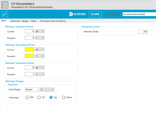
Figure 3: Chronopotentiometry (CP) Experiment Basic Tab in AfterMath
During the induction period, a set of initial conditions are applied to the electrochemical cell and the cell equilibrates at these conditions. Data are not collected during the induction period, nor are they shown on the plot during this period.
After the induction period, the current applied to the working electrode is stepped to the specified value for the duration of the experiment, which is called the electrolysis period. The galvanostatic circuit of the instrument maintains constant applied current while simultaneously measuring the potential at the working electrode relative to the reference electrode. During the electrolysis period, potential and current at the working electrode are recorded at regular intervals as specified on the Basic tab.
The experiment concludes with a relaxation period. During the relaxation period, a set of final conditions (specified on the Advanced tab) are applied to the electrochemical cell and the cell equilibrates at these conditions. Data are not collected during the induction period, nor are they shown on the plot during this period.
A plot of the typical experiment sequence, containing labels of the fields on the Basic tab, helps to illustrate the sequence of events in a CP experiment (see Table 1 and Figure 4).


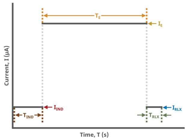
Chronopotentiometry (CP) Basic Tab Field Diagram
At the end of the relaxation period, the post-experiment idle conditions are applied to the cell, and the instrument returns to the idle state. The default plot generated from the data is measured potential vs. time, called a chronoamperogram.
3.2. Advanced Tab
The CP Advanced tab contains two groups for iR Compensation and for Experiment End Trigger (see Figure 5).
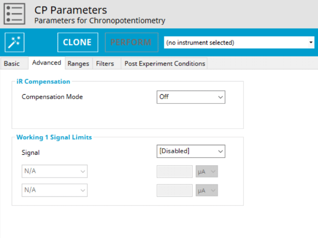
Figure 5: Chronopotentiometry (CP) Experiment Advanced Tab in AfterMath
Detailed description of the iR Compensation Mode is provided elsewhere on the knowledgebase. This mode is used to correct for uncompensated resistance in the electrochemical cell.
In a CP experiment, the researcher might want to have AfterMath monitor the response (input) and then stop the experiment a specific current, potential, and/or charge. This value is called a trigger and is set in the Experiment End Trigger group on the Advanced tab (see Figure 5). For CP, the signals for the trigger can be potential or current. A common example of using this trigger is in the charging of a battery. A researcher would charge the battery by performing a CP experiment (also called a CC or constant current) with the trigger set to its upper potential limit (e.g., 100% SOC). Once this potential limit is reached, the CP experiment terminates and retains the data collected up to the trigger endpoint. More information about end triggers is available on the Knowledgebase.
3.3. Ranges, Filters, and Post Experiment Conditions Tab
The Ranges tab contains the Electrode Range group, which contains the initial current and potential range fields.
These fields are often duplicated, and linked to, the same fields on the Basic tab. Additionally, a field for Autorange control for both potential and current appears on this tab. More information on autorange is available elsewhere on the knowledgebase.
The Filters tab provides access to potentiostat hardware filters, including stability, excitation, current response, and potential response filters. Pine Research recommends that users contact us for help in making changes to hardware filters. Advanced users may have an easier time changing the automatic settings on this tab.
By default, the potentiostat disconnects from the electrochemical cell at the end of an experiment. There are other options available for what these post-experiment conditions can be and are controlled by setting options on the Post Experiment Conditions tab.
4. Sample Data
The typical chronopotentiogram for a 1 mM acetaminophen in saline solution shows a plot similar to a potentiometric titration (see Figure 6). Initially, the potential is slightly rising until nearly all of the acetaminophen at the electrode is consumed, at which point the potential rises rapidly through an inflection point, followed by a trailing off of the potential after the inflection point. AfterMath has many ways to view and analyze data as well as to customize plots.
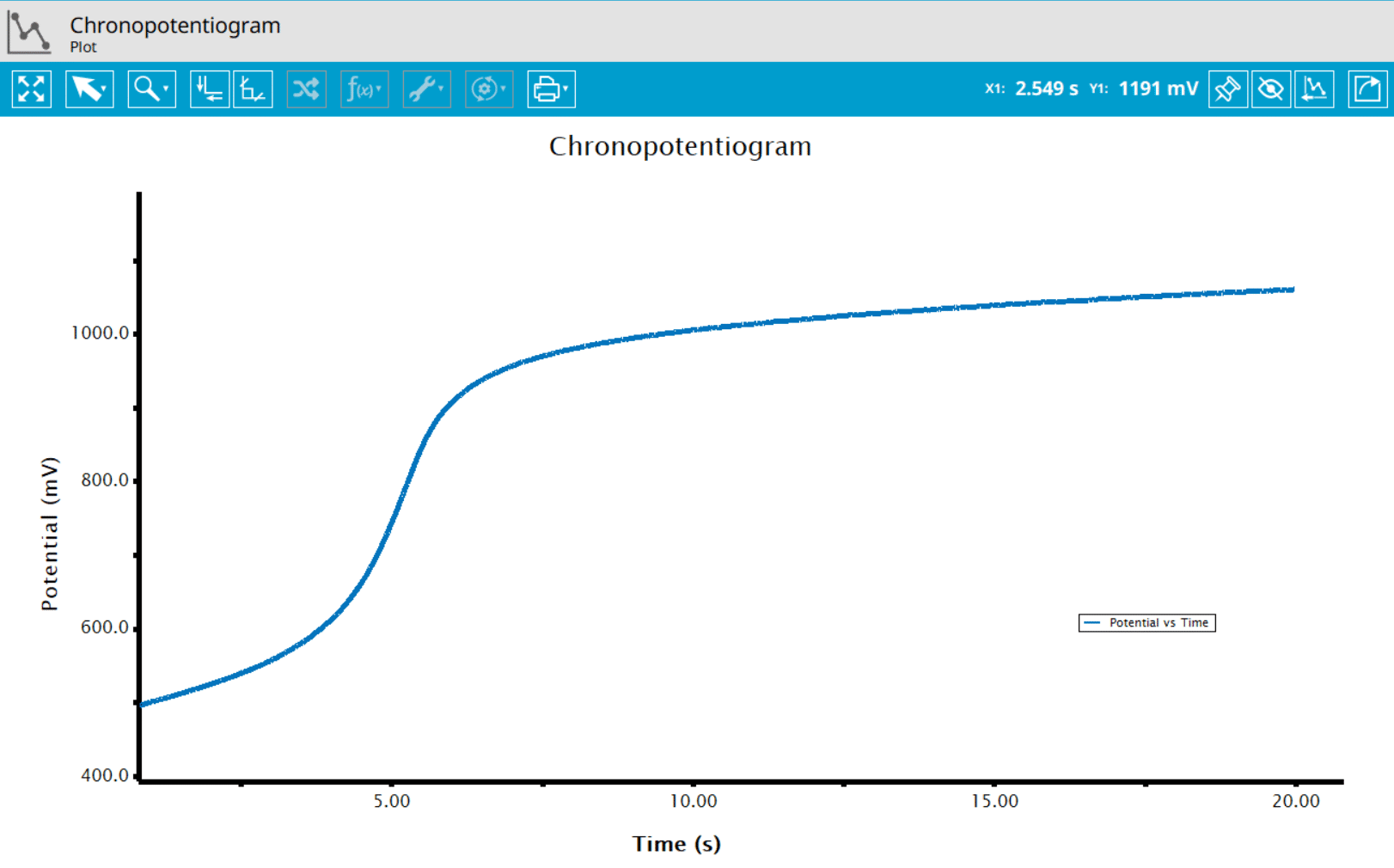
Figure 6: Chronopotentiogram of 1 mM acetaminophen
The addition of a Baseline Tool aids in finding the inflection point, the point at which the slope of the plot is greatest (see Figure 7). Once the tool has been added to the trace on the plot, right-click the tool to view its properties. There, change the baseline mode to Tangent to easily find the inflection point. The potential at 


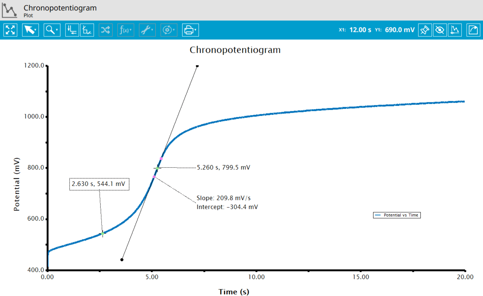
Figure 7: Chronopotentiogram of acetaminophen with inflection point labeled
5. Applications from Literature
Here, CP was used to measure diffusion coefficients. Le et al. generated concentration polarization at an anion exchange membrane under constant current (CP)4. The potential drop across the membrane was monitored as a function of time. By determining the transition time (point of inflection) calculate diffusion coefficients were calculated for several chloride salts in 0.1 M solutions. An exquisite example, considering the authors were able to determine diffusion coefficients of non-redox active species.
In another example, Nagaraju and Lakshminarayanan used CP to grow mesoporous Au films for use in the electro-oxidation of alcohols in alkaline media5. The researchers showed that varying the current density and deposition yielded different surface areas. These films were then used to electro-oxidize methanol or ethanol indicating that they could be used in direct alcohol alkaline fuel cells.
6. References
- Bard, A. J.; Faulkner, L. A. Electrochemical Methods: Fundamentals and Applications, 2nd ed. Wiley-Interscience: New York, 2000.
- Kissinger, P.; Heineman, W. R. Laboratory Techniques in Electroanalytical Chemistry, 2nd ed. Marcel Dekker, Inc: New York, 1996.
- Wang, J. Analytical Electrochemistry, 3rd ed. John Wiley & Sons, Inc.: Hoboken, NJ, 2006.
- Le, X. T.; Viel, P.; Tran, D. P.; Grisotto, F.; Palacin, S. Surface Homogeneity of Anion Exchange Membranes: A Chronopotentiometric Study in the Overlimiting Current Range. The Journal of Physical Chemistry B, 2009, 113(17), 5829-5836.
- Nagaraju, D. H.; Lakshminarayanan, V. Electrochemically Grown Mesoporous Gold Film as High Surface Area Material for Electro-Oxidation of Alcohol in Alkaline Medium. The Journal of Physical Chemistry C, 2009, 113(33), 14922-14926.