Calculating Diffusion Coefficients Using GITT and PITT

1. Intermittent Titration Techniques

Intermittent titration techniques are specialized electrochemical methods commonly used for studying energy storage devices (e.g., batteries, supercapacitors). They also offer the added benefit of enabling measurement of mass transport properties, such as the diffusion coefficient. While these techniques result in the charging and/or discharging of the device under test (DUT), they are not as frequently used for extremely long term or cycled experiments. For those applications, researchers more commonly use galvanostatic charge/discharge (GCD), or what is known to battery researchers as constant current-constant voltage (CC-CV) tests. However, intermittent titration techniques allow a more gradual and controlled study of the DUT’s charge/discharge profile, and the calculation of the diffusion coefficient is an added bonus.

There are two types of intermittent titration techniques: Galvanostatic Intermittent Titration Technique (GITT), and Potentiostatic Intermittent Titration Technique (PITT).

2. Galvanostatic Intermittent Titration Technique (GITT)

In a GITT experiment, current is the controlled variable and voltage (potential) is the measured variable. The experiment consists of repeatedly alternating between an applied current and zero current (i.e., rest, or open circuit) until the measured voltage reaches a desired set point. The times for each step (active duration and rest duration) are often the same and are commonly around 10 to 15 minutes each, but they don’t have to be identical. See Figure 1 below for example of the current vs. time waveform in a typical GITT experiment.

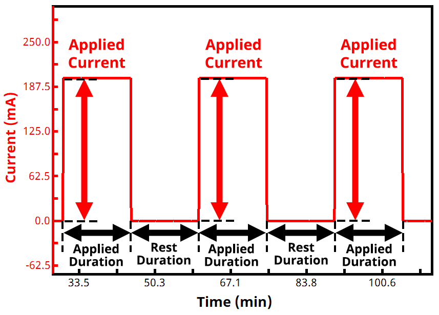
Figure 1. GITT Current vs. Time Waveform

During each active step, the voltage rises or falls (depending whether it is a charging or discharging current being applied), and the voltage then subsequently relaxes during each rest step. As soon as the measured voltage reaches a target value, the experiment either reverses direction with a new target voltage (for a two-segment GITT experiment), or it ends (for a one-segment GITT experiment). GITT experiments with more than two segments are possible but less common.

See Figures 2 and 3 below for examples of current and voltage vs. time GITT waveforms, both for a zoomed in portion of the experiment (Fig. 2) and an entire two-segment GITT test (Fig. 3).

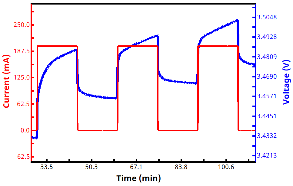
Figure 2. GITT Current and Voltage vs. Time Waveforms Zoomed

Figure 3. Two-Segment GITT Current and Voltage vs. Time Waveforms

While calculations for the applied current and expected charge/discharge rate can be done by the researcher using the specific and/or gravimetric capacity of the DUT, it cannot be exactly known beforehand how long each GITT segment will last. It is therefore also impossible to know exactly how many active and rest steps will be required before the target voltage is reached. This kind of time-agnosticism is typical for GCD and other galvanostatic experiments commonly performed on energy storage devices.

Figure 4 shows an example voltage vs. capacity plot for a two-segment GITT experiment. Since current is being controlled and is constant during each active step, the charge/discharge curves from a GITT experiment consist of equal segments of capacity over the entire voltage window. Vertical lines separating each active segment illustrate the impact of the relaxing voltage during each rest step. (Note: added capacity is zero during each rest step because the current is zero, though the voltage is still changing. This explains the presence of vertical spikes/lines throughout the curves seen in Fig. 4)

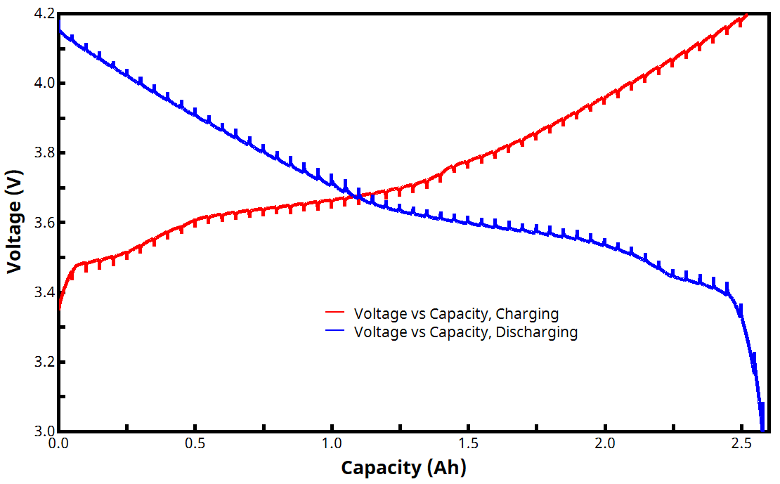
Figure 4. Two-Segment GITT Voltage vs. Capacity Curves

2.1. Diffusion Coefficient Calculation from GITT

Calculation of the diffusion coefficient, $\displaystyle{D}$ , from a GITT experiment is performed automatically in AfterMath Blue software and is determined by the following equation:

$\displaystyle{D = \frac{4}{\pi} {\left( i L\right)}^2 \frac{{\left( \frac{dE}{dQ}\right)}^2}{{\left(\frac{dE}{d\sqrt{t}}\right)}^2}}$

where $\displaystyle{i}$ is the applied current, $\displaystyle{L}$ is the characteristic length, $\displaystyle{{dE}/{dQ}}$ is the slope of voltage vs. capacity (charge), and $\displaystyle{{dE}/{d\sqrt{t}}}$ is the slope of voltage vs. square root of time. Note that the applied current, along with these two slopes, are taken from data measured only during the active steps.

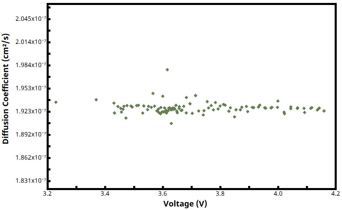
Upon completion of a GITT experiment using a Pine Research potentiostat and AfterMath Blue software, calculated values of $\displaystyle{D}$ for each active step are automatically plotted vs. voltage (see Figure 5 for example plot of $\displaystyle{D}$ vs. voltage).

Figure 5. GITT Diffusion Coefficient vs. Voltage Plot

The characteristic length can be somewhat arbitrary, which can make the diffusion coefficient calculation slightly tenuous. This is because it may not always be clear whether to use the electrode thickness, diameter, or perhaps some other dimension. The researcher is encouraged to consult the literature for guidance regarding selection of characteristic length.

Another aspect of the GITT diffusion coefficient equation shown above is that it is derived based on the assumption of relatively short timescales. Specifically, the criterion is that the time, $\displaystyle{t}$ , must follow the relationship $\displaystyle{t \ll L^2 / D}$ . This can create a slightly tricky proposition: to determine whether the timescale was appropriately small enough to justify calculation of the diffusion coefficient from GITT data, the researcher must first use the same equation to calculate $\displaystyle{D}$ . This is somewhat of a “Catch-22” situation, coupled as well with the uncertainty of selecting the most accurate dimension for $\displaystyle{L}$ as previously mentioned. For these reasons, while it is relatively easy to calculate $\displaystyle{D}$ from GITT experiments, the researcher is encouraged to exercise caution when analyzing the values and make every attempt to verify adherence to the timescale assumption if possible.

3. Potentiostatic Intermittent Titration Technique (PITT)

In a PITT experiment, voltage (potential) is the controlled variable and current is the measured variable. The experiment consists of repeatedly alternating between an applied voltage and rest (i.e., open circuit), with regular applied voltage increments, until a voltage set point is reached. The times for each step (active duration and rest duration) are often the same and are commonly around 10 to 15 minutes each, but they don’t have to be identical. See Figure 6 below for example of the voltage vs. time waveform in a typical PITT experiment.

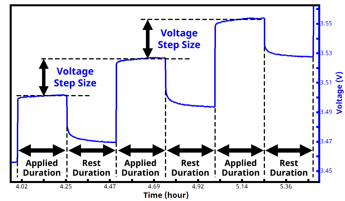
Figure 6. PITT Voltage vs. Time Waveform

During each active step, the measured current is either positive or negative (depending whether it is a charging or discharging PITT segment) and typically decays following a Cottrell-like response. During each subsequent rest step, the voltage relaxes as the circuit is open and the current goes to zero. As soon as the applied voltage reaches a target value, the experiment either reverses direction with a new target voltage (for a two-segment PITT experiment), or it ends (for a one-segment PITT experiment). PITT experiments with more than two segments are possible but less common.

See Figures 7 and 8 below for examples of voltage and current vs. time PITT waveforms, both for a zoomed in portion of the experiment (Fig. 7) and an entire two-segment PITT test (Fig. 8).

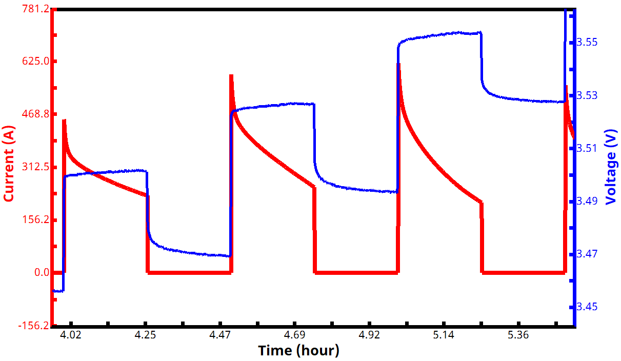
Figure 7. PITT Voltage and Current vs. Time Waveforms Zoomed

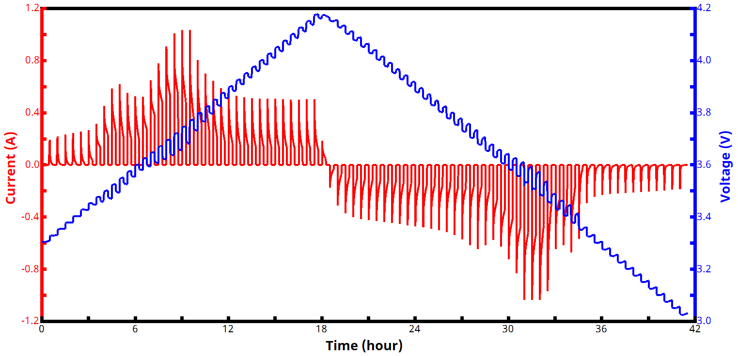
Figure 8. PITT Voltage and Current vs. Time Waveforms

Unlike with a GITT experiment, for a PITT experiment it can be fully known beforehand exactly how many steps (active and rest) will be required to reach the target voltage (the notable exception being if the initial OCV is not yet known, and PITT voltage increments are entered based on this initial OCV). What can be difficult to know beforehand with a PITT experiment, however, is what the measured current responses will be for each applied voltage step. If the voltage increment is too large, the system will reach the target voltage faster (quicker charge/discharge) and the current responses may be aggressively high. Conversely, if the voltage increment is too small, the system will take longer to reach the target voltage (slower charge/discharge) and the current responses may be very small and/or difficult to measure. Since either of these extremes are generally undesirable, trial and error may be required to determine the optimal voltage increment for each PITT segment.

Figure 9 shows an example voltage vs. capacity plot for a two-segment PITT experiment. Since current is not being controlled, and is changing during each active step, the charge/discharge curves from a PITT experiment consist of unequal segments of capacity over the entire voltage window. Vertical lines separating each active segment illustrate the impact of the relaxing voltage during each rest step. (Note: added capacity is zero during each rest step because the current is zero, though the voltage is still changing. This explains the presence of vertical spikes/lines throughout the curves seen in Fig. 9)

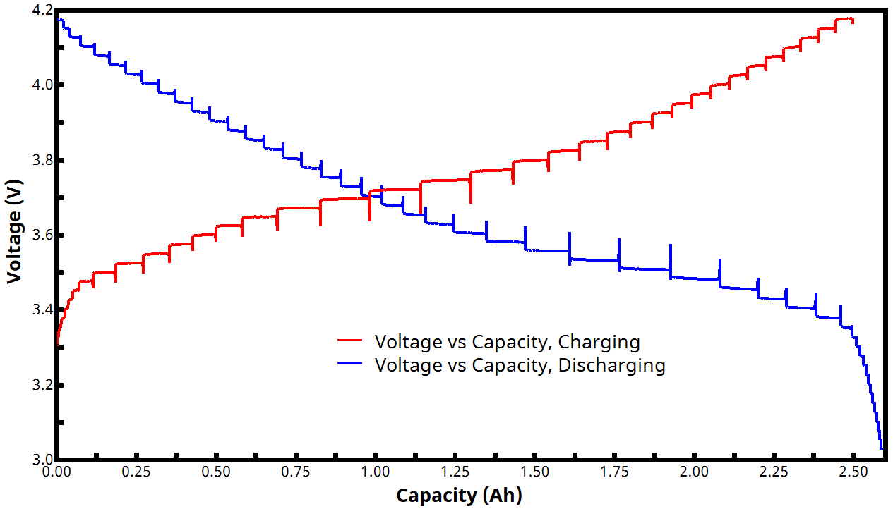
Figure 9. Two-Segment PITT Voltage vs. Capacity Curves

3.1. Diffusion Coefficient Calculation from PITT

Calculation of the diffusion coefficient, $\displaystyle{D}$ , from a PITT experiment is performed automatically in AfterMath Blue software and is determined by the following equation:

$\displaystyle{D = \frac{4L^2}{{\pi}^2} \frac{d \ln i}{dt}}$

where $\displaystyle{L}$ is the characteristic length and $\displaystyle{{d \ln i}/{dt}}$ is the slope of the natural logarithm of the measured current vs. time. Note that this slope is taken from data measured only during the active steps.

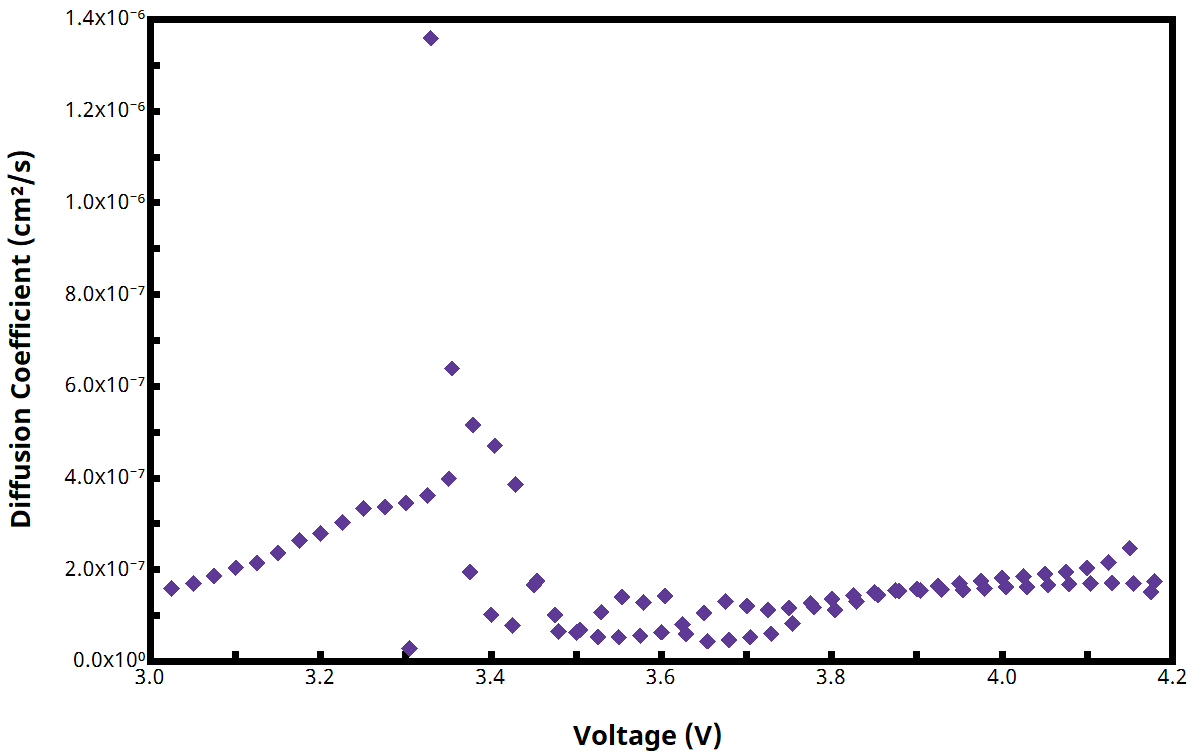
Upon completion of a PITT experiment using a Pine Research potentiostat and AfterMath Blue software, calculated values of $\displaystyle{D}$ for each active step are automatically plotted vs. voltage (see Figure 10 for example plot of $\displaystyle{D}$ vs. voltage).

Figure 10. PITT Diffusion Coefficient vs. Voltage Plot

Another aspect of the PITT diffusion coefficient equation shown above is that it is derived based on the assumption of relatively long timescales. Specifically, the criterion is that the time, $\displaystyle{t}$ , must follow the relationship $\displaystyle{t \gg L^2 / D}$ . This can create a slightly tricky proposition: to determine whether the timescale was appropriately long enough to justify calculation of the diffusion coefficient from PITT data, the researcher must first use the same equation to calculate $\displaystyle{D}$ . This is somewhat of a “Catch-22” situation, coupled as well with the uncertainty of selecting the most accurate dimension for $\displaystyle{L}$ as previously mentioned. For these reasons, while it is relatively easy to calculate $\displaystyle{D}$ from PITT experiments, the researcher is encouraged to exercise caution when analyzing the values and make every attempt to verify adherence to the timescale assumption if possible.

4. References

Wen, C. J.; Boukamp, B. A.; Huggins, R. A.; Weppner, W. Thermodynamic and Mass Transport Properties of “ LiAl .” J. Electrochem. Soc. 1979, 126 (12), 2258. https://doi.org/10.1149/1.2128939.
Xie, J.; Imanishi, N.; Zhang, T.; Hirano, A.; Takeda, Y.; Yamamoto, O. Li-Ion Diffusion Kinetics in LiFePO4 Thin Film Prepared by Radio Frequency Magnetron Sputtering. Electrochimica Acta 2009, 54 (20), 4631–4637. https://doi.org/10.1016/j.electacta.2009.03.007.
Zhu, Y.; Wang, C. Galvanostatic Intermittent Titration Technique for Phase-Transformation Electrodes. J. Phys. Chem. C 2010, 114 (6), 2830–2841. https://doi.org/10.1021/jp9113333.
Cabañero, M. A.; Boaretto, N.; Röder, M.; Müller, J.; Kallo, J.; Latz, A. Direct Determination of Diffusion Coefficients in Commercial Li-Ion Batteries. J. Electrochem. Soc. 2018, 165 (5), A847. https://doi.org/10.1149/2.0301805jes.