What is iR drop?

1. Introduction to iR Compensation

iR drop refers to the decrease in the effective potential applied to the electrochemical double layer. R in iR is often called the uncompensated solution resistance which is the ionic electrolyte resistance between the tip of the reference electrode and the working electrode surface. If iR drop is not accounted for, it can lead to distorted electrochemical data. For example, iR drop will manifest itself as a larger than normal peak splitting between the cathodic and anodic waves in a cyclic voltammogram. In Figure 1, both cyclic voltammograms (A and B) are of 1 mM ferrocene in 10 mM tetrabuytlammonium hexafluorophosphate dissolved in acetonitrile with approximately 530 Ω of uncompensated solution resistance. 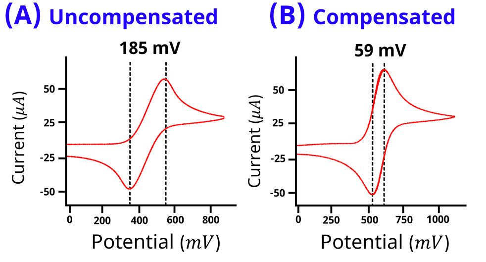A peak splitting $\displaystyle{\Delta E}$ between the oxidation and reduction waves for a kinetically fast 1 electron oxidation reaction of ferrocene is expected to be 59 mV. The solution resistance of 530 Ω is not compensated in Voltammogram A, and a $\displaystyle{\Delta E}$ of 185 mV is observed. Additionally, the measured peak potentials are inaccurate and the duck-shaped voltammogram appears skewed. The solution resistance in voltammogram (B) is compensated, and the peak splitting $\displaystyle{\Delta E}$ is 59 mV.

Cyclic Voltammogram with and without iR compensation

Figure 1: Cyclic voltammogram of 1 mM ferrocene in 10 mM tertrabutylammonium hexafluorophosphate dissolved in acetonitrile without iR compensation (A) and with iR compensation (B). Voltammogram (A) appears tilted with a peak splitting of 185 mV. Voltammogram (B) has no tilt with peak splitting of 59 mV.

iR drop can best be understood when modeling a standard 3-electrode system as a circuit. A standard 3-electrode system consists of a working electrode, counter electrode, and reference electrode, in an electrolyte solution, which can be modeled as a Randle’s Circuit (see Figure 2). The potentiostat connects to the electrochemical cell via the working drive (red), working sense (orange), counter (green), and reference electrode (white) leads. The applied potential/current is driven between the working drive and the counter electrode leads.

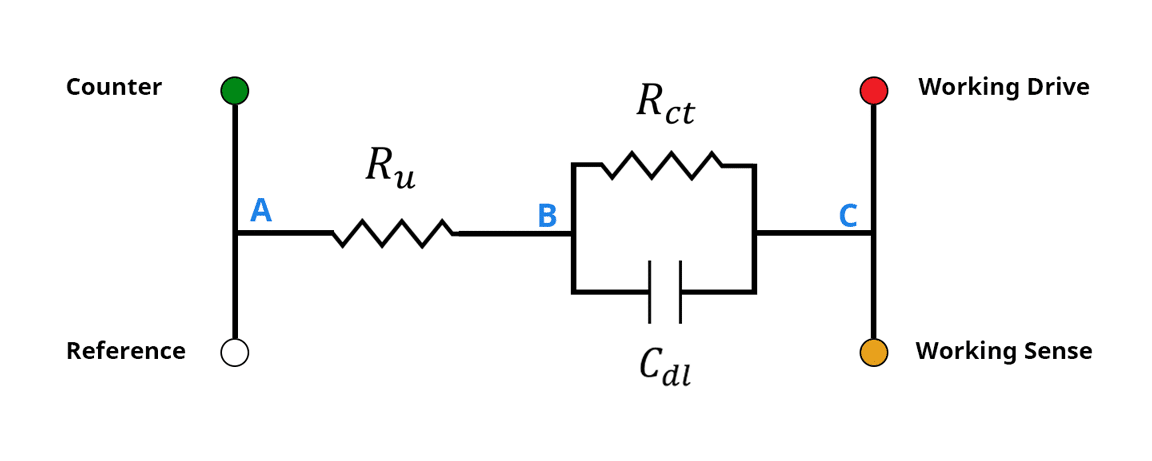
Randles circuit and potentiostat leads. Rct represents the charge transfer resistance and Cdl represents the capacitance of the electrical double-layer at the electrode/electrolyte interface. Ru represents the uncompensated solution resistance.

Figure 2: Randles circuit and potentiostat leads. Rct represents the charge transfer resistance and Cdl represents the capacitance of the electrical double-layer at the electrode/electrolyte interface. Ru represents the uncompensated solution resistance.

The measured potential/current is made between the working sense and reference leads. The working electrode/electrolyte interface is modeled by $\displaystyle{C_{dl}}$ and $\displaystyle{R_{ct}}$ in parallel, where $\displaystyle{C_{dl}}$ is the electrochemical double layer capacitance and $\displaystyle{R_{ct}}$ is the charge transfer resistance associated with a redox reaction. In Figure 2, the solution resistance between points A and B is modeled as a resistor $\displaystyle{R_u}$ . The iR drop refers to Ohm's law (Equation 1), where the current ( $\displaystyle{i}$ ) times $\displaystyle{R_u}$ represents the voltage drop that the potentiostat has to compensate.

$\displaystyle{V=R_u \times i}$

(3)

Electrochemists are interested in measuring the potential across the electrode/electrolyte interface, between points B and C in Figure 2. When modeling with a circuit, one could imagine using a digital multimeter to measure the potential between points B and C. However, within an electrochemical system, this is not practical because, although point A can be connected to directly, point B is difficult if not impossible to access. As a result, there is always an $\displaystyle{R_u}$ that is part of the measurement. When $\displaystyle{R_u}$ is small, it doesn't make a large impact on the accuracy of our measurement, as is the case with most aqueous electrolyte systems. When $\displaystyle{R_u}$ and/or $\displaystyle{i}$ is large, the electrode potential measurements can contain a large iR error. You can also find our video description of iR drop on our YouTube channel.

2. How to Correct for Ohmic Drop

We recommend that scientists make adjustments to their experiment or the instrument to correct for iR drop before experimentation. Correcting for iR drop can be made after an experiment, but it is difficult to correct data in post-processing. Most potentiostats can correct for uncompensated solution resistance by adjusting the potentiostat feedback mechanism. This procedure is known as iR compensation, which requires that the solution resistance is known and entered into the potentiostat software. However, it is advised that before adjusting the potentiostat for iR compensation, the user should attempt to change the physical conditions of their electrochemical system if possible. Some methods for reducing the iR drop include

Increasing the electrolyte concentration to increase solution conductivity
Minimize the solution distance between the reference and working electrode
Decrease the working electrode area to decrease the current.

If adjustments to the electrochemical system are not practical, iR compensation can be activated to correct for the iR drop. The first step is to determine the value of the uncompensated solution resistance accurately. Below we describe several potentiostat techniques that can determine the uncompensated solution resistance, which can also be watched on our YouTube channel.

2.1. Electrochemical Impedance Spectroscopy

Electrochemical Impedance Spectroscopy (EIS) is an AC electroanalytical chemistry technique where a potentiostat applies a sinusoidal potential (or current) and measures a sinusoidal current (or potential). The ratio of the frequency-dependent potential over the frequency-dependent current gives us the impedance. For a complete understanding of EIS, we recommend you check out our other knowledgebase article on the . Section 3 in particular describes how circuit modeling can be used to determine the impedance of specific elements in a Randles circuit. From section 3.2 of our EIS basics knowledgebase article, the total impedance of our Randles circuit (Figure 2) can be described by Equation 2 below.

$\displaystyle{Z_{\omega}= R_u+\frac{R_{ct}}{1+R_{ct}C_{dl}(j\omega)}}$

(4)

When the frequency $(\Omega)$ is large, the denominator in the fraction $\displaystyle{Z_{\omega}= R_u+\frac{R_{ct}}{1+R_{ct}C_{dl}(j\omega)}}$

becomes very large and the fraction approaches 0. This leaves the impedance at high frequency to equal ${R_u}$ . Current will take the path of least resistance, and it has to pass through ${R_u}$ , but it could go through either ${R_u}$ or ${C_{dl}}$ . Because the capacitor ${C_{dl}}$ acts as a short circuit at high frequencies, the only resistance (or impedance) the current experiences is through ${R_u}$ . Experimentally, ${R_u}$ is calculated by performing several high frequency EIS experiments and averaging the results. EIS is one of the best techniques for measuring ${R_u}$ , but not all potentiostats are capable of doing EIS. Pine Research offers several potentiostats capable of doing EIS, the and the . The remaining techniques listed below do not require EIS, and can be performed by a potentiostat that only has DC techniques.

2.2. Current Interrupt

Current Interrupt is a technique for measuring the iR drop by applying a constant current to the electrochemical system followed by disconnecting (interrupting) the counter electrode. The potentiostat measures the potential as a function of time, and at the point where the counter electrode is disconnected ${(t=0)}$ , the potential drops by ${i \times R_u}$ (Figure 3).

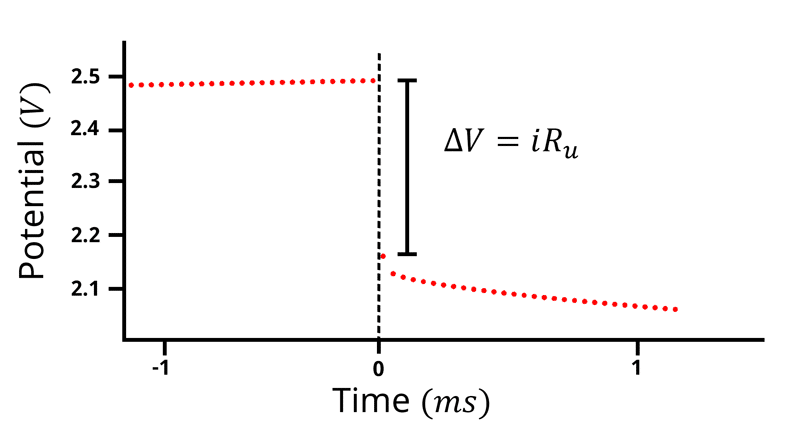
Figure 3: Potential vs time plot of the current interrupt technique. A current of 1 mA is applied while the potential is measured as a function of time. At t=0, the counter electrode lead is disconnected, and the potential drops by the amount of the current (1 mA) times the uncompensated solution resistance.

In Figure 2, when a constant current passes between points A and C, the capacitor ${C_{dl}}$ gets charged. The total potential of the system, measured between A and C in Figure 2, is equal to the sum of the potential of the electrolyte interface (between B and C) and the potential from the uncompensated solution resistance (between A and B), ${i \times R_u}$ . If the current suddenly drops to 0, the potential across ${R_u}$ instantaneously goes to 0. However, the potential across the electrochemical interface (between B and C), does not drop to 0, and decays slowly as the capacitor discharges. Specifically, the potential decays according to the RC time constant. For example, if ${R_{ct}}$ is thousands of ohms, and the ${C_{dl}}$ is on the order of 1-2 μF (for a 5 mm OD glassy carbon electrode), then the RC time constant is roughly several milliseconds, meaning it takes a few milliseconds for 36.8% of its initial state of charge to discharge. If it takes several milliseconds for the circuit to discharge, the potentiostat must sample the potential much faster than the rate of discharging. In this case, the sample rate should be at least tens of microseconds. When the potential is sampled quickly enough, the first few points after the current is interrupted should be used to calculate the iR drop. There are a few instances where the first few data points contain errors, for example, when cable capacitance is an error source. As a result, ${R_u}$ is sometimes determined by extrapolating the RC decay curve to the ${t=0}$ point, and using the extrapolated potential value at ${t=0}$ to calculate the iR drop.

2.3. Potential Step

The potential step technique for determining the iR drop is particularly suited to the situation where it is difficult to pass a large current as required by the current interrupt technique. Rather than applying a constant current followed by an interruption, potential step is a chronoamperometry experiment, where a constant applied potential is followed by a sudden step at ${t=0}$ .

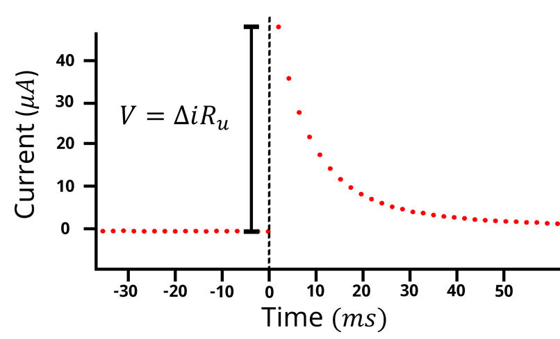
Figure 4: Current vs time plot for a potential step experiment. The potential is kept at an equilibrium value so little to no current flows, followed by a potential step, resulting in a spike in the current which then decays over time. The iR drop is equal to the difference in current at t=0 times the solution resistance.

When the potential is stepped at ${t=0}$ the ${C_{dl}}$ will start to charge and effectively act like a short circuit. This is similar to calculating ${R_u}$ with EIS, where ${C_{dl}}$ has very low impedance at high frequency. At ${t=0}$ , ${C_{dl}}$ appears as a short circuit. The current will choose the path of lease resistance, avoiding ${R_{ct}}$ . The resulting current spike at ${t=0}$ is associated with ${R_u}$ (see Figure 4).

2.4. Positive Feedback

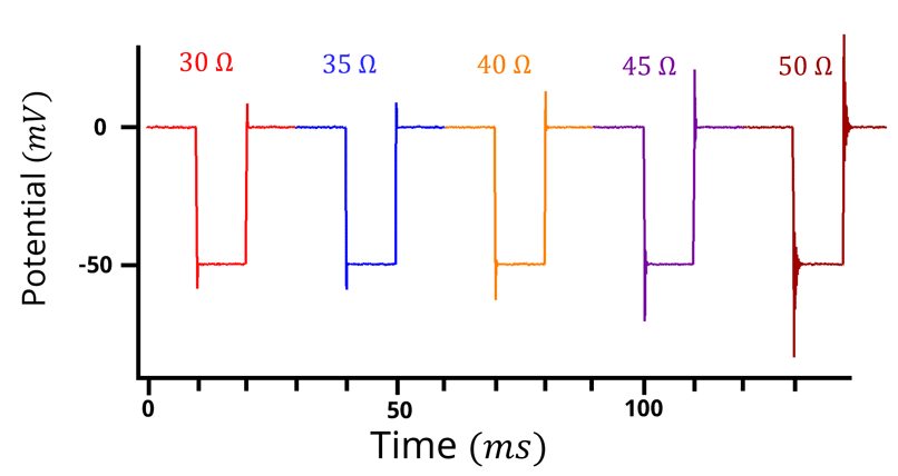
The purpose of determining ${R_u}$ is to activate iR compensation in your potentiostat to compensate for the iR drop. iR compensation requires a positive feedback loop which tends to cause the potentiostat to become unstable or to oscillate. Thus, the best and most practical technique for determining the best R is to apply a series of test R values found before the potentiostat goes into oscillation (Figure 5). The best R value should be entered into the potentiostat software in any subsequent experiment where iR compensation mode is turned on.

Figure 5: Potential vs time plot for a positive feedback experiment. 50 mV potential step, 5 Ohm increment. with 20 ms step duration. As the resistance increases, oscillation/ringing occurs at the edge of the potential step.

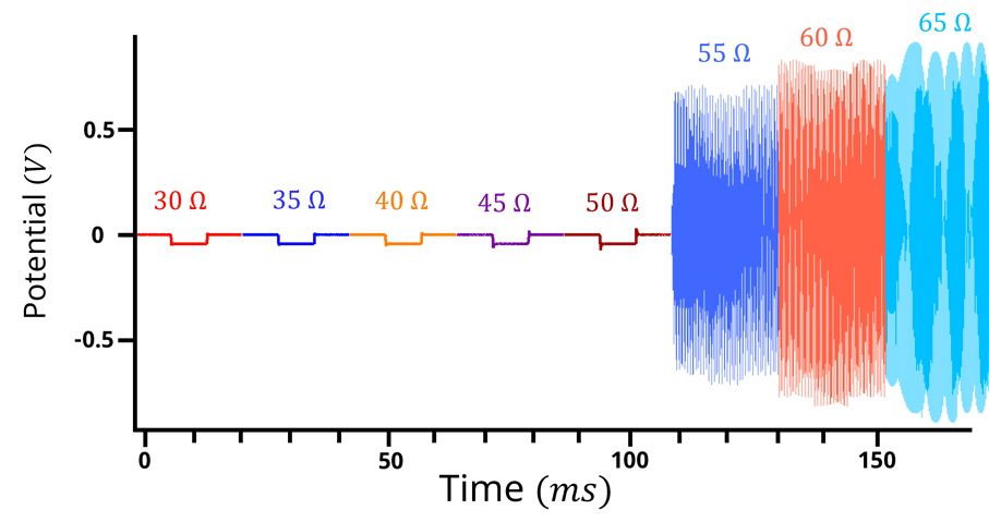
In the positive feedback experiment, the user selects a range of ${R_u}$ values either based on prior experience or on the estimated value determined using another technique (e.g. the previously mentioned techniques). In Figure 5, the range is between 30 - 50 Ω. For each potential step, the ${R_u}$ is increased until the entire range of ${R_u}$ values have been probed. As the potential is stepped and the ${R_u}$ correction is applied, the edges of the potential step will start to oscillate. If the edges of the potential step oscillate too much (Figure 6) then you have overcompensated for the ${R_u}$ .

Figure 6: Potential vs time plot for a positive feedback experiment with too much oscillation. 50 mV potential step, 5 Ohm increment. with 20 ms step duration. At 55 Ohms and beyond, potentiostat overcompensates.

In the above case, selecting 45 Ω or 50 Ω would be a good selection for the ${R_u}$ . However, there are scenarios where the ${R_u}$ value is completely unknown and the value could range from 0 - 5000 Ω. Hypothetically, let's assume the ${R_u}$ is 1345 Ω, but we the researcher didn't know that. If positive feedback was performed from 0 - 5000 Ω with 5 Ω increments and each increment took 20 ms (the parameters used in Figure 6), the total experiment would take a little over 3 minutes to complete. Determining the ${R_u}$ could be faster if several positive feedback experiments were performed. In the example above, if a 100 Ω increment was used, the experiment would be completed in 10 seconds. During the 10-second experiment, oscillations are initially observed between 1200 and 1500 Ohms. 1200-1500 Ohms is too large a range to know the ${R_u}$ value, hence a second positive feedback experiment between 1200 – 1500 Ω with a 5 Ω increment at 20 ms step would be performed. This experiment takes 12 seconds, and the second positive feedback experiment shows oscillation starting around 1340-1350 Ω. At this point 1345 Ω could be selected as ${R_u}$ .

Help us curate the best support content. Give us a thumbs up if helpful, or a thumbs down if not helpful.