AfterMath Electrochemical Studio Simulation – Verification

Last Updated: 3/30/23 by Tim Paschkewitz

Article Contents/Section Navigation

1Simulation Model and Engine Verification

In using any new software, users might be skeptical or uncertain about what the software reports. We have found it very helpful to compare the output from our simulation software to the classic examples found in the 3rd Edition of Electrochemical Methods by Bard, Faulkner, and White.

2AfterMath Electrochemical Studio Simulation Basics

Before you delve into AfterMath Electrochemical Studio Simulation it will be helpful to know a few things about our implementation. Perhaps it's true in all niche areas of science, but electrochemistry seems especially riddled with unclear semantics, labels, interpretations, and positions:

Oxidation is to the right (unless it's to the left).
Cathodic current is positive (unless it's negative).
Potential goes on the x-axis (unless it goes on the y-axis), and it increases positively to the right (unless it increases negatively to the right, if it even belongs on the horizontal axis).
Homogenous rate constant in the forward direction, for a quasi-reversible reaction, is k_f (unless it's k_b, unless it's k₁).
Butler-Volmer kinetics should always be used (unless you should always use Marcus-Hush).
Elementary charge transfer reactions transfer only one electron at a time (unless they can transfer n electrons at a time).
When it comes to α, it is only for the forward reaction and there's no corollary (unless there's a 1 - α corollary), and it's never labeled as anything but α (unless it's labeled α_C or α_A).
Polarographic plotting convention is the only correct choice (unless you plot in IUPAC convention).

Here at Pine Research, we are like the rest of the community. We pick a position and firmly plant our feet into it. We know we won't get it right for all of you, but our goal is to be as clear as possible about what we have done. We do not want to force conventions or labels onto you, but we also have to pick something. We consider it our job to make our choices abundantly clear to you as the user. That said, here are some choices we made in Simulation, which are important to know. We wrote a separate article about this so that when you can be made adequately aware of our choices.

3Recreations of Electrochemical Methods Figures

We simulated the following examples in AfterMath Electrochemical Studio. The plots were customized (colors, weights, fonts, etc.) in AfterMath to resemble the examples in the text. In all cases, the output from our simulations exactly matches the cases provided in the text.

As with all things electrochemistry, labels for parameters are not always the same across the landscape. In AfterMath Electrochemical Studio, we have landed on the following labels found in Simulation:

Label	Description
k⁰	Heterogeneous electron transfer rate for a quasi-reversible or irreversible charge transfer reaction (in units of cm/s).
k₁	Homogeneous rate constant for a quasi-reversible chemical reaction in the forward direction (1° units s^-1, 2° units M^-1s^-1). Sometimes the label k_f is used.
k_-1	Homogeneous rate constant for a quasi-reversible chemical reaction in the backwards direction (1° units s^-1, 2° units M^-1s^-1). Sometimes the label k_b is used.
K_eq	Homogeneous rate constant for a fully reversible chemical reaction (at fast equilibrium) (unitless). This is the only condition where K_eq is explicitly defined. With quasi-reversible chemical reactions, K_eq is calculated as $\displaystyle{K_{eq}=\frac{k_{1}}{k_{-1}}}$ and displayed for reference.
k	Homogeneous rate constant for an irreversible chemical reaction in (only) the forward direction (1° units s^-1, 2° units M^-1s^-1). Sometimes the label k_f is used.

NOTE: By default, AfterMath Electrochemical Studio follows the IUPAC plotting convention, which is increasing positive potential (x-axis) to the right, increasingly positive current (y-axis) up (anodic current, oxidation), increasingly negative current (y-axis) down (cathodic current, reduction). Electrochemical Methods primarily uses the polarographic plotting convention, which is increasing positive potential (x-axis) to the left, increasingly positive current (y-axis) up (cathodic current, reduction), increasingly negative current (y-axis) down (anodic current, oxidation). Below, we have adjusted the default display from AfterMath Electrochemical Studio to match what is shown in Electrochemical Methods.

3.1Figure 13.3.1 (a - d) - ErCi Mechanism

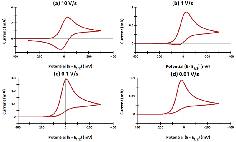
Figure 13.3.1 (a - d). Cyclic Voltammogram for the E_rC_i Case as a Function of Sweep Rate.

The EC mechanism is shown on Page 553. Figure 13.3.1 describes a specific case of EC with a reversible electrochemical reaction and irreversible chemical reaction (E_rC_i). For this example, Cyclic Voltammograms were generated from the following reaction:

E_r

$A+e \rightleftharpoons B$

(1)

C_i

$B \rightarrow C$

(2)

With the following simulation parameters:

Reaction Dynamics

Reaction	E⁰ (mV)	k⁰ (cm/s)	α	k₁ (s^-1)	k_-1 (s^-1)	k (s^-1)
1	0	∞	0.5	-	-	-
2	-	-	-	-	-	10

Species Details

Species	*C (mM)**	D (cm²/s)
A	1	10^-5
B	0	10^-5
C	0	10^-5

Cyclic Voltammetry Sweep Parameters

Parameter	Value
Segments	2
Initial Potential (V)	0.4
Vertex Potential (V)	-0.3
Final Potential (V)	0.3
Sweep Rate (V/s)	a) 10 b) 1 c) 0.1 d) 0.01

Experiment Variables

Parameter	Value
Diffusion Type	Linear (1D)
Electrode Area (cm²)	1
Temperature (°C)	25
Concentration	Use Bulk Concentrations (C*)
Double-Layer Capacitance (F)	-
Uncompensated Resistance (Ω)	-

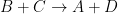
3.2Figure 13.3.1 (e) - ErCi Mechanism (Dimensionless Current)

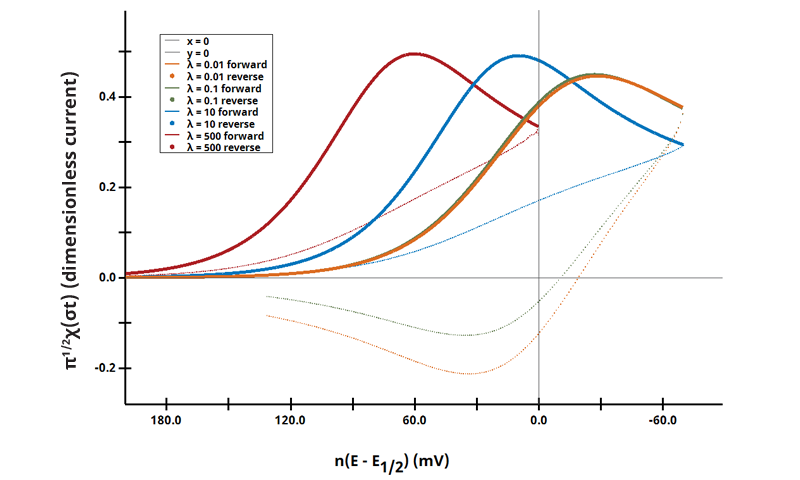
Figure 13.3.1 (e). Voltammetric Response of an ErCi Mechanism in Terms of λ and Dimensionless Current.

The EC mechanism is shown on Page 553. Figure 13.3.1 (e) shows the use of dimensionless kinetic parameter λ and dimensionless current as a function of Χ(σt) (see Equation 7.2.18 on page 315 ):

$\displaystyle{\chi(\sigma t)=\frac{g(z)}{C_{O}^{*}\left(\pi D_{O}\sigma \right)^{1/2}}=\frac{i(\sigma t)}{nFAC_{O}^{*}\left(\pi D_{O}\sigma \right)^{1/2}}}$

Cyclic Voltammograms were generated with the same reaction as above; however as a function of λ = 500, 10, 0.1, and 0.01. The benefit of visualizing data like these is to understand a range of kinetic behaviors and their effects on a single comparison plot.

3.3Figure 13.3.4 - ErCiEr Mechanism

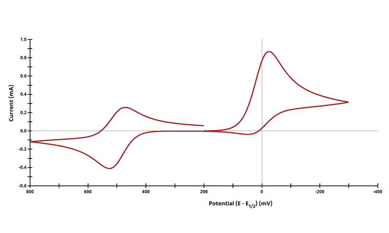
Figure 13.3.4 Cyclic Voltammogram for the E_rC_i Case.

The ECE mechanism is shown on Page 556. Figure 13.3.4 describes a specific case of ECE with a two reversible electrochemical reactions and irreversible chemical reaction (E_rC_i). For this example, Cyclic Voltammograms were generated from the following reaction:

E_r

$A+e \rightleftharpoons B$

(1)

C_i

$B \rightarrow C$

(2)

E_r

$C+e \rightleftharpoons D$

(3)

With the following simulation parameters:

Reaction Dynamics

Reaction	E⁰ (mV)	k⁰ (cm/s)	α	k₁ (s^-1)	k_-1 (s^-1)	k (s^-1)
1	0	∞	0.5	-	-	-
2	-	-	-	-	-	10
1	500	∞	0.5	-	-	-

Species Details

Species	*C (mM)**	D (cm²/s)
A	1	10^-5
B	0	10^-5
C	0	10^-5
D	0	10^-5

Cyclic Voltammetry Sweep Parameters

Parameter	Value
Segments	3
Initial Potential (V)	0.2
Upper Potential (V)	0.8
Lower Potential (V)	-0.3
Final Potential (V)	0.2
Sweep Rate (V/s)	1

Experiment Variables

Parameter	Value
Diffusion Type	Linear (1D)
Electrode Area (cm²)	1
Temperature (°C)	25
Concentration	Use Bulk Concentrations (C*)
Double-Layer Capacitance (F)	-
Uncompensated Resistance (Ω)	-

3.4Figure 13.3.9 - ErCi' Mechanism

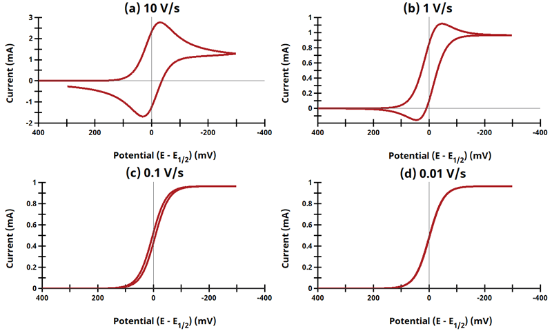
Figure 13.3.9 - Cyclic Voltammograms for the E_rC_i' Case.

The EC' mechanism is shown on Page 562. Figure 13.3.9 describes a specific case of EC' (catalytic) with a reversible electrochemical reactions and irreversible chemical reaction (E_rC_i'). For this example, Cyclic Voltammograms were generated from the following reaction:

E_r

$A+e \rightleftharpoons B$

(1)

C_i'

$B+C \rightarrow A+D$

(2)

What is unique about EC' reactions is that the product from the electrochemical reaction (B) can chemically react with excess substrate (C) to regenerate the initial species (A). Since species C is in large excess relative to A/B, we can ignore the diffusion of C and the reaction kinetics are treated as pseudo first order in B as $\displaystyle {rate=k'[B]}$ . AfterMath Electrochemical Studio detects the conditions of an EC' reaction, and when the substrate is adequately higher in concentration than the starting species from the charge transfer reaction, the software will invoke the pseudo first-order kinetics approximation, where $\displaystyle{rate=k_1[B][C] \left(\text{in units of}\;M^{-1}s^{-1}\right)\Rightarrow rate=k'[B] \left(\text{in units of}\; s^{-1}\right)}$ by taking $k_1 \times C_C^{*} = k'$ . The following simulation parameters were used:

Reaction Dynamics

Reaction	E⁰ (mV)	k⁰ (cm/s)	α	k₁ (s^-1)	k_-1 (s^-1)	k (M^-1s^-1)
1	0	1000	0.5	-	-	-
2	-	-	-	-	-	10

Species Details

Species	*C (mM)**	D (cm²/s)
A	1	10^-5
B	0	10^-5
C	1000	10^-5
D	0	10^-5

Cyclic Voltammetry Sweep Parameters

Parameter	Value
Segments	2
Initial Potential (V)	0.4
Vertex Potential (V)	-0.3
Final Potential (V)	0.3
Sweep Rate (V/s)	a) 10 b) 1 c) 0.1 d) 0.01

Experiment Variables

Parameter	Value
Diffusion Type	Linear (1D)
Electrode Area (cm²)	1
Temperature (°C)	25
Concentration	Use Bulk Concentrations (C*)
Double-Layer Capacitance (F)	-
Uncompensated Resistance (Ω)	-

3.5Figure 13.3.10 - ErCi' Mechanism (Dimensionless Current)

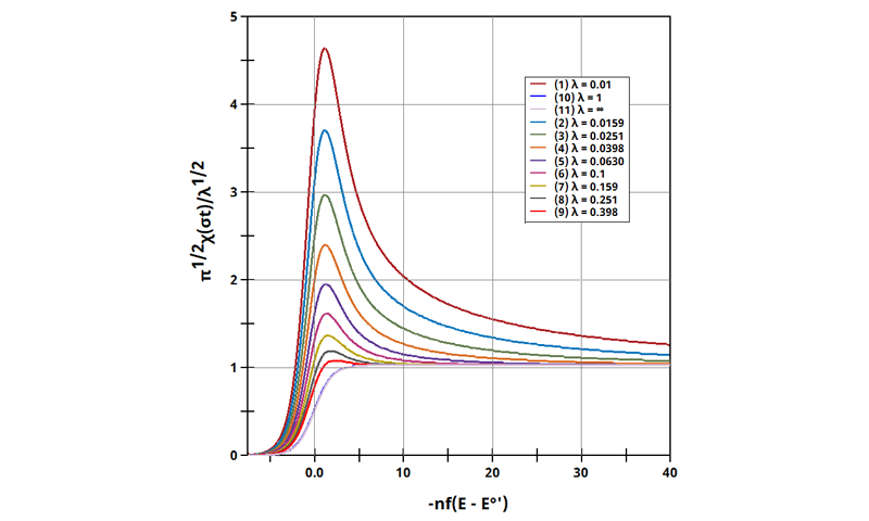
Figure 13.3.10 Linear Sweep Voltammogram for the E_rC_i' Case using Dimensionless Current.

The EC' mechanism is shown on Page 562. Figure 13.3.10 describes a specific case of EC' (catalytic) with a reversible electrochemical reactions and irreversible chemical reaction (E_rC_i'). For this example, current was used to interrogate the system as a function of $\displaystyle{\lambda=k_1C_C^{*}/nf\nu}$ . Linear Sweep Voltammograms were generated with real current and potential, whose variables were determined with this calculation of λ. The following real parameters and conditions were used to generate the data in this plot:

E_r

$A+e \rightleftharpoons B$

(1)

C_i'

$B+C \rightarrow A+D$

(2)

Reaction Dynamics

Reaction	E⁰ (mV)	k⁰ (cm/s)	α	k₁ (s^-1)	k_-1 (s^-1)	k (M^-1s^-1)
1	0	∞	0.5	-	-	-
2	-	-	-	-	-	38.9426

$k$ was calculated by assuming a series of sweep rates, shown below, and used as a constant for each trace.

Species Details

Species	*C (mM)**	D (cm²/s)
A	1	10^-5
B	0	10^-5
C	1000	10^-5
D	0	10^-5

Cyclic (Linear Sweep) Voltammetry Sweep Parameters

Parameter	Value
Segments	1
Initial Potential (V)	0.1926
Final Potential (V)	-1.027
Sweep Rate (V/s)	see below

Experiment Variables

Parameter	Value
Diffusion Type	Linear (1D)
Electrode Area (cm²)	1
Temperature (°C)	25
Concentration	Use Bulk Concentrations (C*)
Double-Layer Capacitance (F)	-
Uncompensated Resistance (Ω)	-

Dimensionless Terms

Case	λ	k (M^-1s^-1)	ν (V/s)
1	1.00 × 10^-2	38.9426	100.00
2	1.59 × 10^-2	38.9426	62.89
3	2.51 × 10^-2	38.9426	39.56
4	3.98 × 10^-2	38.9426	24.88
5	6.30 × 10^-2	38.9426	15.65
6	1.00 × 10^-1	38.9426	9.84
7	1.59 × 10^-1	38.9426	6.19
8	2.51 × 10^-1	38.9426	3.89
9	3.98 × 10^-1	38.9426	2.45
9	1.00	38.9426	0.1
10	∞	38.9426	0.001

3.6Figure 13.3.13 - CrEr Mechanism

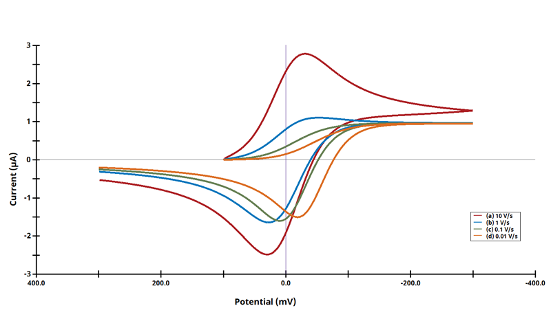
Figure 13.3.13 Linear Sweep Voltammogram for the C_rE_r Case using Dimensionless Current.

The CE' mechanism is shown on Page 566. Figure 13.3.13 describes a specific case of CE with a reversible chemical and reversible electrochemical reaction (C_rE_r). The following real parameters and conditions were used to generate the data in this plot:

C_R

$A \rightleftharpoons B$

(1)

E_r

$B+e \rightleftharpoons C$

(2)

To recreate this plot, Pre-Equilibrium concentrations must be used to ensure that there is adequate concentration of C present to show the immediate oxidation wave. By default, bulk concentrations (C*) are used in AfterMath Electrochemical Studio. Making assumptions about equilibration can lead to erroneous results and should be avoided. Alas, there are times when the model may not adequately compute fractional concentrations near the electrode interface in coupled mechanisms. Since all reactions happen at the same time, everywhere, some users may wish to assume Nernstian equilibrium previails at the onset of the simulation, thereby making select species (initially absent) having a very small but non-zero fractional concentration at t = 0. Users can select "Use Equilibrium Concentrations [C]" on the Settings tab of Simulation, to enable equilibrium concentration calculated values for initial concentrations (instead of the bulk provided on the Mechanism tab). To exactly re-create the figure, we have used Equilibrium concentrations for the data in the plot above. The following simulation parameters were used:

Reaction Dynamics

Reaction	E⁰ (mV)	k⁰ (cm/s)	α	k₁ (s^-1)	k_-1 (s^-1)	k (M^-1s^-1)
1	-	-	-	0.01	10	-
2	0	∞	0.5	-	-

Species Details

Species	*C (mM)**	D (cm²/s)
A	1	10^-5
B	0	10^-5
C	0	10^-5

Cyclic (Linear Sweep) Voltammetry Sweep Parameters

Parameter	Value
Segments	2
Initial Potential (V)	0.1
Vertex Potential (V)	-0.3
Final Potential (V)	0.3
Sweep Rate (V/s)	a) 10 b) 1 c) 0.1 d) 0.01

Experiment Variables

Parameter	Value
Diffusion Type	Linear (1D)
Electrode Area (cm²)	1
Temperature (°C)	25
Concentration	Use Equilibrium Concentrations [C]
Double-Layer Capacitance (F)	-
Uncompensated Resistance (Ω)	-

3.7Figure 13.3.16 - ErEr Mechanism

Figure 13.3.16 Cyclic Voltammograms for the E_rE_r Case.

The EE mechanism is shown on Page 570. Figure 13.3.16 describes a series of two reversible electrochemical reactions whose $\displaystyle{\Delta E^{0}=E_2^{0}-E_1^{0}}$ varies (E_rE_r). The following real parameters and conditions were used to generate the data in these plots:

E_r

$A+e \rightleftharpoons B$

(1)

E_r

$B+e \rightleftharpoons C$

(2)

Readers may recall that this series of cyclic voltammograms was on the cover of Electrochemical Methods, 2nd Edition. The following simulation parameters were used:

Reaction Dynamics

Reaction	E⁰ (mV)	k⁰ (cm/s)	α	k₁ (s^-1)	k_-1 (s^-1)	k (M^-1s^-1)
1	a) 0 b) 0 c) 0 d) 35.6 e) 75 f) 90 g) 110 h) 150 i) 200	100	0.5	-	-	-
2	a) 100 b) 50 c) 0 d) 0 e) 0 f) 0 g) 0 h) 0 i) 0	100	0.5	-	-	-

Species Details

Species	*C (mM)**	D (cm²/s)
A	1	10^-5
B	0	10^-5
C	0	10^-5

Cyclic (Linear Sweep) Voltammetry Sweep Parameters

Parameter	Value
Segments	2
Initial Potential (V)	0.5
Vertex Potential (V)	-0.2
Final Potential (V)	0.5
Sweep Rate (V/s)	0.1

Experiment Variables

Parameter	Value
Diffusion Type	Linear (1D)
Electrode Area (cm²)	1
Temperature (°C)	25
Concentration	Use Bulk Concentrations (C*)
Double-Layer Capacitance (F)	-
Uncompensated Resistance (Ω)	-

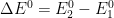
3.8Figure 13.3.20 - ErEq Mechanism

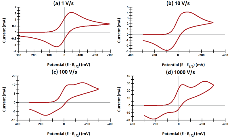
Figure 13.3.20 Cyclic Voltammograms for the E_rE_q Case.

The EE mechanism is shown on Page 574. Figure 13.3.20 describes a series of a reversible electrochemical reaction and a quasi-reversible electrochemical reaction where any effect of disproportionation/comproportionation were excluded (i.e., rate constants for the reaction $\displaystyle{A+C \rightarrow 2B}$ = 0). The following real parameters and conditions were used to generate the data in these plots:

E_r

$A+e \rightleftharpoons B$

(1)

E_q

$B+e \rightleftharpoons C$

(2)

Reaction Dynamics

Reaction	E⁰ (mV)	k⁰ (cm/s)	α	k₁ (s^-1)	k_-1 (s^-1)	k (M^-1s^-1)
1	0	∞	0.5	-	-	-
2	0	0.01	0.5	-	-	-

Species Details

Species	*C (mM)**	D (cm²/s)
A	1	10^-5
B	0	10^-5
C	0	10^-5

Cyclic (Linear Sweep) Voltammetry Sweep Parameters

Parameter	Value
Segments	2
Initial Potential (V)	0.3
Vertex Potential (V)	-0.3
Final Potential (V)	0.3
Sweep Rate (V/s)	a) 1 b) 10 c) 100 d) 1000

Experiment Variables

Parameter	Value
Diffusion Type	Linear (1D)
Electrode Area (cm²)	1
Temperature (°C)	25
Concentration	Use Bulk Concentrations (C*)
Double-Layer Capacitance (F)	-
Uncompensated Resistance (Ω)	-

3.9Figure 13.3.21 - ErEq Mechanism

Figure 13.3.21 Cyclic Voltammograms for the E_rE_q Case.

The EE mechanism is shown on Page 575. Figure 13.3.21 describes a series of a reversible electrochemical reaction and a quasi-reversible electrochemical reaction where any effect of disproportionation/comproportionation were excluded (i.e., rate constants for the reaction $\displaystyle{A+C \rightarrow 2B}$ = 0). In these simulation, $\displaystyle{\Delta E^{0}=150 \; mV}$ The following real parameters and conditions were used to generate the data in these plots:

E_r

$A+e \rightleftharpoons B$

(1)

E_q

$B+e \rightleftharpoons C$

(2)

Readers may recall that in Electrochemical Methods, 2nd Edition, this same figure was erroneously duplicated from a previous figure. During testing of AfterMath Electrochemical Studio Simulation, this error was noticed and mentioned to the authors, who subsequently updated this figure in the 3rd Edition.

Reaction Dynamics

Reaction	E⁰ (mV)	k⁰ (cm/s)	α	k₁ (s^-1)	k_-1 (s^-1)	k (M^-1s^-1)
1	0	∞	0.5	-	-	-
2	0.15	0.01	0.5	-	-	-

Species Details

Species	*C (mM)**	D (cm²/s)
A	1	10^-5
B	0	10^-5
C	0	10^-5

Cyclic (Linear Sweep) Voltammetry Sweep Parameters

Parameter	Value
Segments	2
Initial Potential (V)	0.4
Vertex Potential (V)	-0.4
Final Potential (V)	0.4
Sweep Rate (V/s)	a) 1 b) 10 c) 100 d) 1000

Experiment Variables

Parameter	Value
Diffusion Type	Linear (1D)
Electrode Area (cm²)	1
Temperature (°C)	25
Concentration	Use Bulk Concentrations (C*)
Double-Layer Capacitance (F)	-
Uncompensated Resistance (Ω)	-

3.10Figure 13.3.22 - EqEr Mechanism

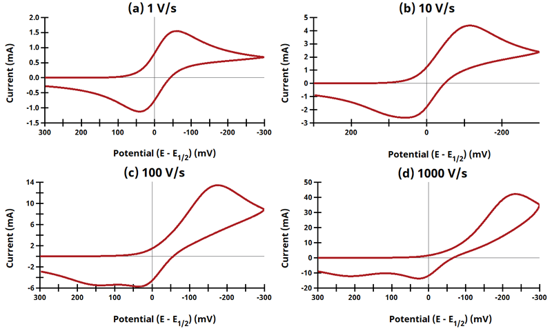
Figure 13.3.22 Cyclic Voltammograms for the E_qE_r Case.

The EE mechanism is shown on Page 576. Figure 13.3.21 describes a series of a quasi-reversible electrochemical reaction and a reversible electrochemical reaction where any effect of disproportionation/comproportionation were excluded (i.e., rate constants for the reaction $\displaystyle{A+C \rightleftharpoons 2B}$ = 0). The following real parameters and conditions were used to generate the data in these plots:

E_q

$A+e \rightleftharpoons B$

(1)

E_r

$B+e \rightleftharpoons C$

(2)

Reaction Dynamics

Reaction	E⁰ (mV)	k⁰ (cm/s)	α	k₁ (s^-1)	k_-1 (s^-1)	k (M^-1s^-1)
1	0	0.01	0.5	-	-	-
2	0	∞	0.5	-	-	-

Species Details

Species	*C (mM)**	D (cm²/s)
A	1	10^-5
B	0	10^-5
C	0	10^-5

Cyclic (Linear Sweep) Voltammetry Sweep Parameters

Parameter	Value
Segments	2
Initial Potential (V)	0.3
Initial Potential (V)	-0.3
Final Potential (V)	0.3
Sweep Rate (V/s)	a) 1 b) 10 c) 100 d) 1000

Experiment Variables

Parameter	Value
Diffusion Type	Linear (1D)
Electrode Area (cm²)	1
Temperature (°C)	25
Concentration	Use Bulk Concentrations (C*)
Double-Layer Capacitance (F)	-
Uncompensated Resistance (Ω)	-

3.11Figure 13.3.25 - ErCiEr Mechanism

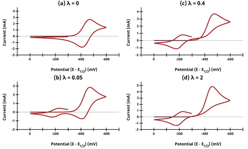
Figure 13.3.25 Cyclic Voltammograms for the E_rC_iE_r Case.

The ECE mechanism is shown on Page 579. Figure 13.3.25 describes a series of a reversible electrochemical reaction, irreversible chemical reaction, and a reversible electrochemical reaction as a function of dimensionless kinetic parameter λ, where $\displaystyle{\lambda = \frac{k_1}{f\nu}}$ . The following real parameters and conditions were used to generate the data in these plots:

E_r

$A+e \rightleftharpoons B$

(1)

C_i

$B \rightarrow C$

(2)

E_r

$C+e \rightleftharpoons D$

(3)

Reaction Dynamics

Reaction	E⁰ (V)	k⁰ (cm/s)	α	k₁ (s^-1)	k_-1 (s^-1)	k (M^-1s^-1)
1	-0.44	∞	0.5	-	-	-
2	-	-	-	-	-	$f(\lambda)$ *
3	-0.2	∞	0.5	-	-	-

*Refer to table below for values of k for a given λ.

Dimensionless Kinetic Parameter, λ

k (s^-1)	λ	f (V^-1)	ν (V/s)
0	0	38.922	10
19.461	0.05	38.922	10
155.687	0.4	38.922	10
778.435	2	38.922	10

Species Details

Species	*C (mM)**	D (cm²/s)
A	1	10^-5
B	0	10^-5
C	0	10^-5
D	0	10^-5

Cyclic (Linear Sweep) Voltammetry Sweep Parameters

Parameter	Value
Segments	3
Initial Potential (V)	0
Upper Potential (V)	0
Lower Potential (V)	-0.6
Final Potential (V)	-0.3
Sweep Rate (V/s)	10

Experiment Variables

Parameter	Value
Diffusion Type	Linear (1D)
Electrode Area (cm²)	1
Temperature (°C)	25
Concentration	Use Bulk Concentrations (C*)
Double-Layer Capacitance (F)	-
Uncompensated Resistance (Ω)	-

How can we help? What do you want to learn? Search our knowledgebase.

Electrochemical Simulation

AfterMath Electrochemical Studio Simulation – Verification

RELATED AFTERMATH LINKS

RELATED PAGES

Article Contents/Section Navigation

1Simulation Model and Engine Verification

2AfterMath Electrochemical Studio Simulation Basics

3Recreations of Electrochemical Methods Figures

3.1Figure 13.3.1 (a - d) - ErCi Mechanism

3.2Figure 13.3.1 (e) - ErCi Mechanism (Dimensionless Current)

3.3Figure 13.3.4 - ErCiEr Mechanism

3.4Figure 13.3.9 - ErCi' Mechanism

3.5Figure 13.3.10 - ErCi' Mechanism (Dimensionless Current)

3.6Figure 13.3.13 - CrEr Mechanism

3.7Figure 13.3.16 - ErEr Mechanism

3.8Figure 13.3.20 - ErEq Mechanism

3.9Figure 13.3.21 - ErEq Mechanism

3.10Figure 13.3.22 - EqEr Mechanism

3.11Figure 13.3.25 - ErCiEr Mechanism

Questions? Find Answers.

Software

Applications

Theory

Product Specifications