WaveDriver Simple EIS Test
Last Updated: 1/9/23 by Alex Peroff

ARTICLE TAGS
-
WaveDriver test,
-
EIS test
1WaveDriver Simple EIS Test
This test simulates the EIS response of a real electrochemical system involving inductive, resistive, and capacitive elements. A representative circuit containing these elements is built into the EIS Calibration & Dummy Cell
and may be used to test the EIS functionality of the WaveDriver as well as the circuit fitting tools available in the AfterMath software package.
This test is performed during the system testing of a Pine Research WaveDriver potentiostat (WaveDriver 200
and WaveDriver 100
models).
1.1Connect to the EIS Calibration & Dummy Cell
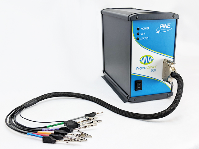
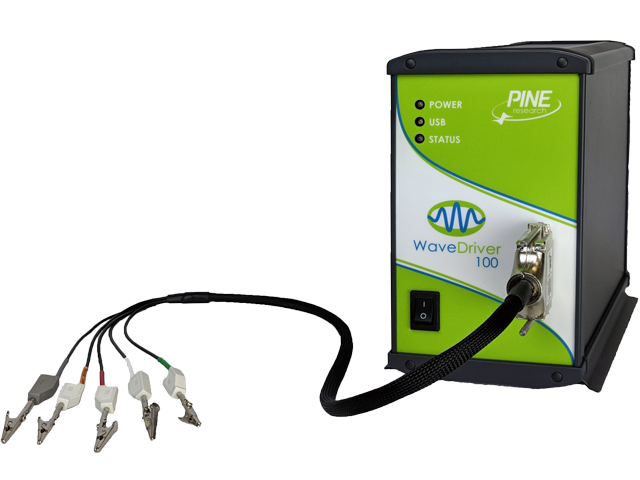
Connect the cell cable to the connector on the front panel of the WaveDriver. Remove all of the alligator clips from the cell cable and insert each banana plug into the proper banana jack on the EIS Calibration & Dummy Cell as shown (see Figure 1). Match the color of each lead to the banana jack with the corresponding color on Row “EIS” of the dummy cell.
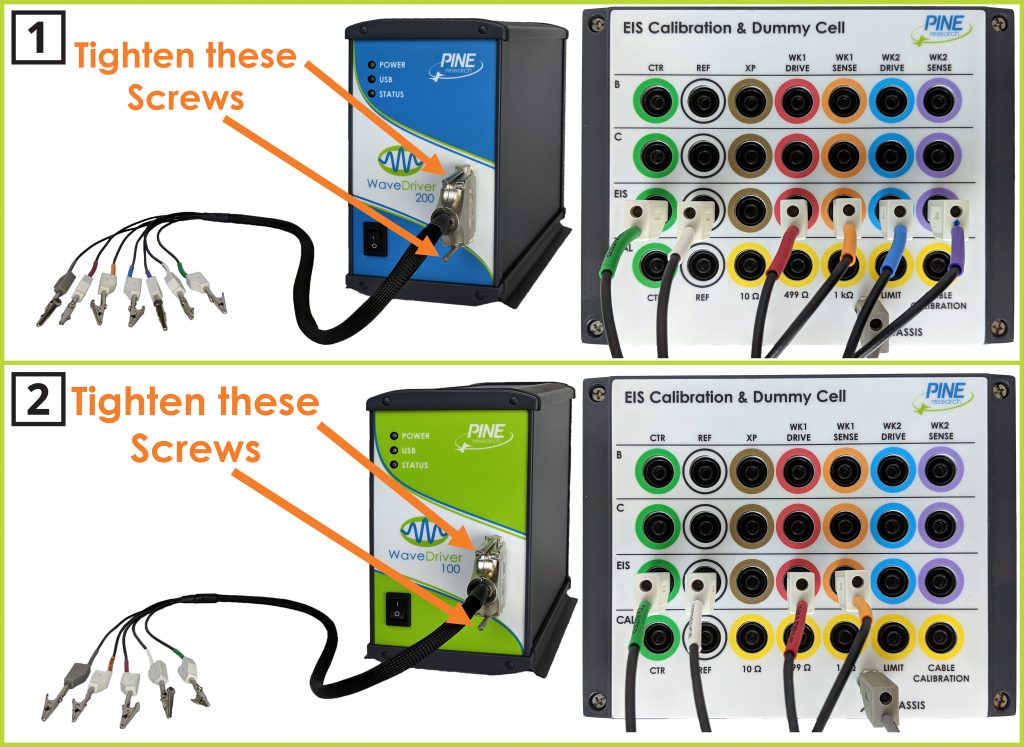
Figure 1. Connections for a Simple EIS Test for (1) WaveDriver 200; and (2) WaveDriver 100
1.2Create a Potentiostatic EIS Experiment (EIS-POT)
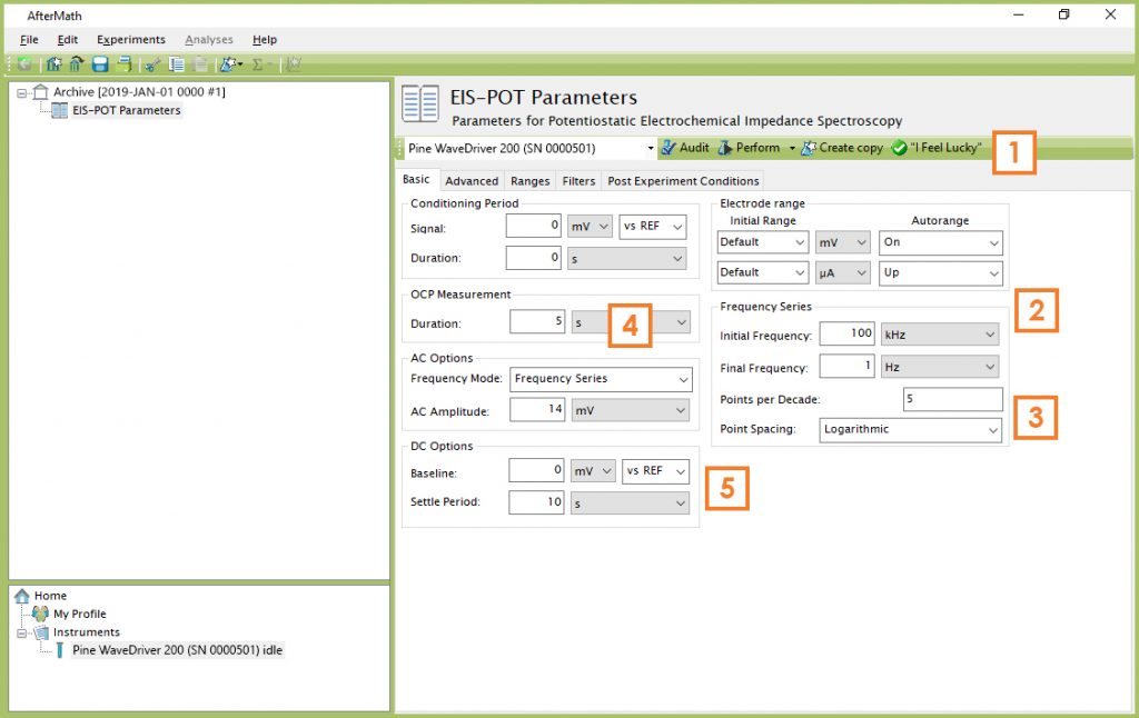
Choose the Potentiostatic Electrochemical Impedance Spectroscopy (EIS-POT) option from the Impedance Spectroscopy sub-menu in the AfterMath Experiments menu. A new EIS-POT specification will be created and placed into the archive. Configure the parameters as shown (see Figure 2).
| 1 |
Click on the “I Feel Lucky” button. Note that default parameters for OCP Measurement Duration, AC Amplitude, DC Baseline, and Frequency Series appear automatically. |
| 2 |
Set the Initial Frequency to 100 kHz; set the Final Frequency to 1 Hz |
| 3 |
Set the Points per Decade to 5 |
| 4 |
Set the OCP Measurement Duration to 5 s |
| 5 |
Set the DC Options Settle Period to 10 s and change the Baseline to “vs REF” |
Figure 2. Experimental Parameters for a Simple EIS Test
TIP: The "I Feel Lucky" button has been renamed "AutoFill" in versions of AfterMath later than May 2019. Newer versions may appear with this change in terminology; however, the functionality of the button remains the same.
1.3Audit Experimental Parameters
Choose the WaveDriver in the drop-down menu (see Figure 3, to the left of the “Audit” button). Press the “Audit” button to check the parameters. AfterMath will perform a quick audit of the parameter values to ensure that all required parameters have been specified and are within allowed ranges.
1.4Initiate the Experiment
Click on the “Perform” button to initiate the EIS-POT experiment. The “Perform” button is located to the right of the “Audit” button (see Figure 3).
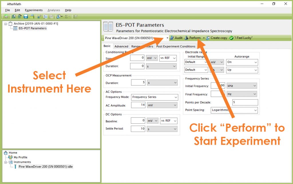
Figure 3. Location of Instrument Selection Menu and Perform Button (EIS-POT)
1.5Monitor Experimental Progress
Monitor the progress of the EIS-POT Simple AC Test experiment in AfterMath by observing the real time plot and the progress bar (see Figure 4). The default live display shows Lissajous plots, but Bode or Nyquist plots can also be observed in real time if desired. Data is automatically updated on these additional plots in real time as the experiment progresses.
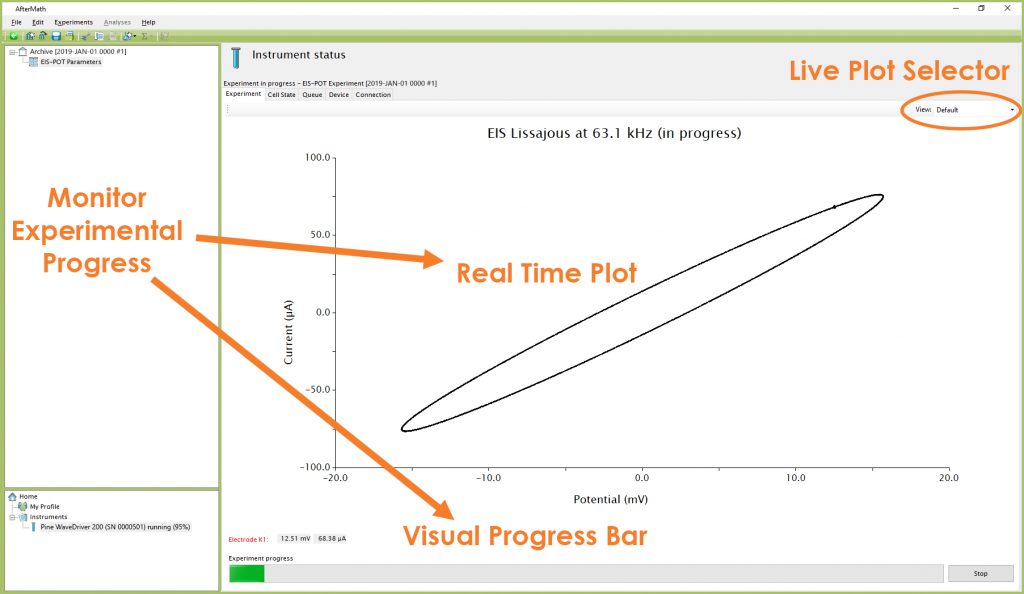
Figure 4. Monitoring the Progress of the EIS-POT Simple AC Test Experiment
NOTE: During an EIS-POT experiment, the percentage complete value displayed at the bottom left portion of the screen refers to each individual frequency and is not indicative of the overall experimental progress.
1.6Review the Results
When the experiment has finished, the results of the experiment are placed in a folder within the archive (see Figures 5 and 6).
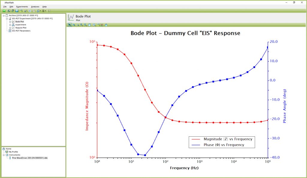
Figure 5. Anticipated EIS-POT Results – Bode Plot (using Dummy Cell Row “EIS”)
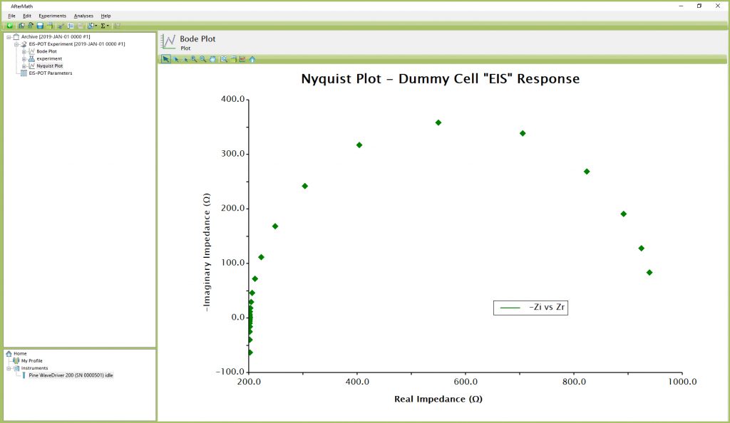
Figure 6. Anticipated EIS-POT Results – Bode Plot (using Dummy Cell Row “EIS”)
In addition to the Bode and Nyquist plots that are automatically populated after an EIS-POT experiment has completed, additional data can be viewed in the “results” node under the “experiment” node of the EIS-POT experiment (see Figure 7). Tabular data can be selected from the drop-down list for all typical EIS parameters, as well as Conditioning Period, Measured OCP, DC Settling Period, and Lissajous results for all applied frequencies. If desired, graphical plots can also be quickly generated for any of the aforementioned tabular data by clicking the “Create Plot” button (see Figure 7).
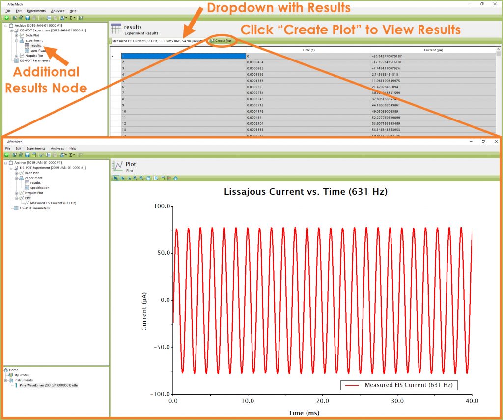
Figure 7. Additional Results Node from EIS-POT Simple AC Test Experiment
1.7Understanding the Results
The representative circuit in Row “EIS” of the EIS Calibration & Dummy Cell contains inductive, resistive, and capacitive elements.
A leading resistor (200 Ω) and inductor (100 μH) represent the uncompensated resistance and inductance that may be present in an actual electrochemical cell. The EIS response observed in the Bode Plot at high frequencies (>~3 kHz) shows how the leading inductor generates a positive (inductive) phase angle while the observed impedance magnitude (~200 Ω) is largely due to the leading resistor (see Figure 5). The influence of the leading inductor is also evident in the Nyquist plot where a negative imaginary impedance is observed (see Figure 6). The intercept with the real impedance axis (~200 Ω) is mainly due to the leading resistor.
In the middle-to-low frequencies on the Bode Plot (between ~3 kHz and 1 Hz), the parallel resistor (750 Ω) and capacitor (22 μF) generate a dip to negative (capacitive) phase angle values as well as an increase in the impedance magnitude. This resistor and capacitor in parallel (i.e., a “parallel RC” element) leads to a characteristic semicircle shape in the Nyquist plot (see Figure 6). The width of this semicircle (measured along the horizontal axis) is a measure of the resistance in the parallel RC element (~750 Ω).
1.8Performing a Circuit Fit Analysis
A Circuit Fit Analysis can be performed on the results to verify the circuit element parameters. Highlight an entry within the EIS-POT experiment in AfterMath and click on either “Analyses” or the “Σ” symbol at the top of the screen and select the “Circuit Fit” option from the menu (see Figure 8).
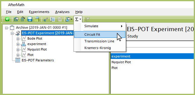
Figure 8. Location of Circuit Fit Analysis in AfterMath
A new Circuit Fit Analysis will be added to the archive. Choose the circuit in the “Built-In Circuits” library which has the title “L1sR1s(Q1pR2)” (see Figure 9).
The circuit schematic diagram will appear to the right of the list. Click the box labeled “OK” to choose this circuit.
Note that this circuit library interface allows the user to either select one of several built-in circuits, or construct a custom circuit model. Details related to these features, as well as a description of the circuit model syntax in AfterMath, can be found elsewhere on the Pine Research Knowledgebase.
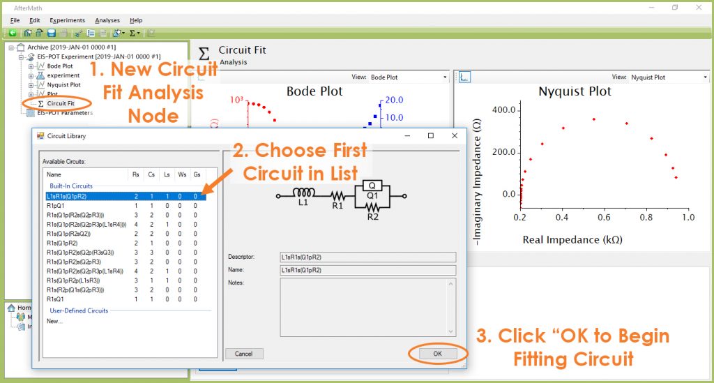
Figure 9. AfterMath Circuit Library Selection for Circuit Fit Analysis
TIP: In AfterMath circuit model syntax, an “s” between two elements indicates a series connection and a “p” indicates a parallel connection. “L” represents an inductor, “R” represents a resistor, and “Q” represents a constant phase element. Circuit elements are numbered uniquely and sequentially. Additionally, the order of connections follows standard mathematical parentheses rules.
Once the circuit has been selected, AfterMath chooses suitable initial “seed” values for each of the circuit parameters, and then the circuit fit is also automatically performed. The Bode and Nyquist Plots on the display are updated to overlay the circuit fit results (computed values) on top of the original experimental data. In some cases, the initial values are sufficient to provide a satisfactory fit (see Figure 10). The user may also view all fitted parameter values along with associated uncertainties on the Calculated Values tab (see Figure 11).
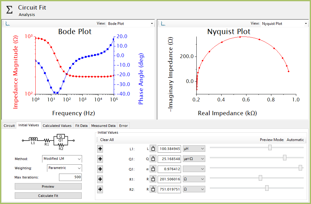
Figure 10. Circuit Fit Analysis Results for EIS Dummy Cell
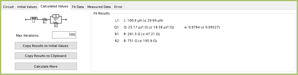
Figure 11. Circuit Fit Calculated Values Tab with Parameter Values and Uncertainties
While the automatically-calculated fit is often acceptable, occasionally it is necessary to iteratively refine the fitted parameter values. AfterMath provides an easy way to accomplish this task. Ideally, each successive iteration moves the parameter values closer to a better overall fit. AfterMath also provides several different fitting methods and weighting options, and sometimes it is helpful to toggle these settings while searching for the best fit. Trial-and-error using multiple fitting methods and weighting options is sometimes required to obtain a satisfactory fit.
To iterate further without changing the fitting method, simply use the “Calculate Fit” button on the Initial Values tab, or the “Calculate More” button on the Calculated Values tab (in conjunction with the “Max Iterations” parameter), to apply as many additional iterations as desired. If further iterations do not appear to refine the overall fit, then it may be necessary to change the fitting method or weighting option being used. To do this, press the “Copy Results to Initial Values” button located on the Calculated Values tab (see Figure 11). This copies the most recent fit results back to the Initial Values tab and allows the fitting method and/or weighting option to be changed. Several fitting methods (Levenberg-Marquardt, Simplex, and Powell) and weighting options (Parametric, Unity, Custom) are available.
1.9Saving the Fitting Results
For the representative circuit in Row “EIS” of the EIS Calibration & Dummy Cell, the circuit fitting process should converge quickly on a good fit after a few iterations. Each of the parameter values produced by the fitting process can be compared to the known values for the resistors, capacitor, and inductor in the representative circuit.
After the fitting process converges on a satisfactory result, the values of the fitting parameters may be copied to the system clipboard using the “Copy Results to Clipboard” button located on the Calculated Values tab (see Figure 11). In addition, duplicate copies of the Bode and Nyquist plots can be copied to the archive by right-clicking the plots and choosing the “Duplicate Plot” option.


 WaveDriver 200 EIS Bipotentiostat/Galvanostat
and WaveDriver 100
WaveDriver 200 EIS Bipotentiostat/Galvanostat
and WaveDriver 100
 WaveDriver 100 EIS Potentiostat/Galvanostat
models).
WaveDriver 100 EIS Potentiostat/Galvanostat
models).