Square Wave Voltammetry (SWV)

Last Updated: 1/5/23 by Alex Peroff

ARTICLE TAGS

AfterMath SWV,
osteryoung,
square wave,
square wave voltammetry,
SWV

CAPABLE POTENTIOSTATS

AFTERMATH LINKS

Article Contents/Section Navigation

1Technique Overview

Square Wave Voltammetry (SWV) is a potentiostatic method that offers some advantages to common techniques like Cyclic Voltammetry (CV), in that the waveform is a series of pulses increasing along a linear baseline, where current is measured in a forward pulse and reverse pulse. The result is the current difference between forward and reverse pulses. The way in which the current is measured at each pulse aids in minimizing the measurement of background (charging) current. Related pulse-type methods include Normal Pulse Voltammetry (NPV) and Differential Pulse Voltammetry (DPV).

Square wave voltammetry (SWV) combines the aspects of several pulse voltammetric methods, including the background suppression and sensitivity of differential pulse voltammetry (DPV), the diagnostic value of normal pulse voltammetry (NPV), and the ability to interrogate products directly in the manner of Reverse NPV.

In an SWV experiment, the potential of the working electrode is stepped through a series of forward and reverse pulses from an initial potential to a final potential. The forward step is determined by the square amplitude and the reverse step is determined by subtracting the square increment from the square amplitude. Cyclic Square Wave Voltammetry (CSWV) is a variant where the potential of the working electrode is cycled between an Upper potential and a Lower potential.

In the simplest case, when Segments (S_N) = 1 (see Figure 1), potential pulses in a forward and reverse pulse, along a linearly increasing baseline from an initial to final potential, sampling current at specified intervals (see Figure 2).

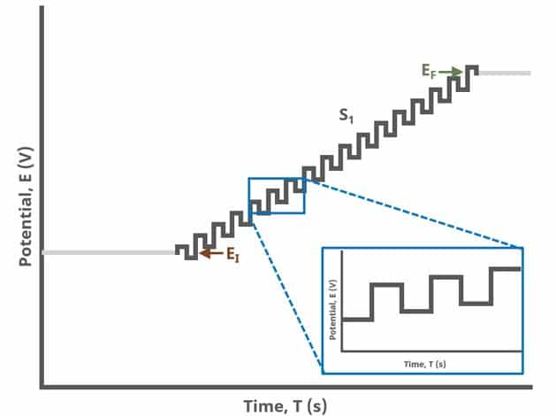
Figure 1. Square Wave Voltammetry (SWV) One Segment Waveform

During each forward or reverse pulse, current is sampled at the same period within the pulse duration as set by entering Sampling width (T_{SW, W}) into the Basic tab (see below). The period of a pulse (T_{SW, P}) includes both forward and reverse pulses; thus, the current sampled in the forward pulse is at,

$\displaystyle {\frac{1}{2}T_{SW,\; P}-T_{SW, \; W}}$

and the current is sampled in the reverse pulse at,

$\displaystyle {T_{SW,\; P}-T_{SW, \; W}}$

as shown in Figure 2.

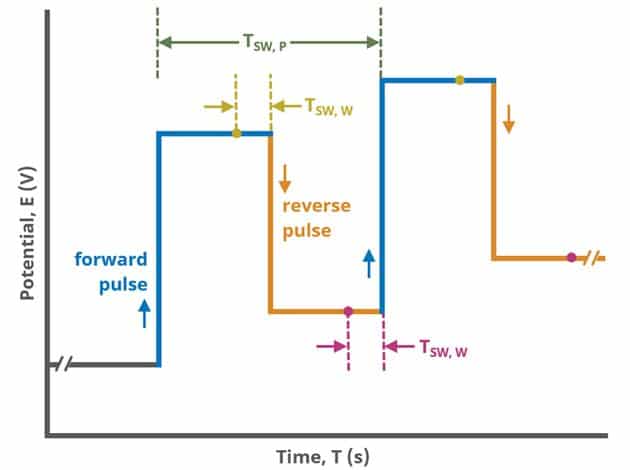
Square Wave Voltamemtry Forward and Reverse Pulse Sampling Diagram

Figure 2. Square Wave Voltammetry Forward and Reverse Pulse Sampling Diagram

In a later Section (Experimental Setup in AfterMath - Basic Tab), the pulse parameters are defined in detail (see Table 1 and Figure 7).

When Segments (S_N) = 2 (see Figure 3), potential pulses in a forward and reverse pulse, along a linearly increasing baseline from an initial potential to vertex potential and then to final potential, sampling current at specified intervals (see Figure 2).

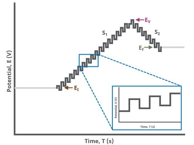
Figure 3. Square Wave Voltammetry (SWV) Two Segment Waveform

When Segments (S_N) = 3 (see Figure 4), potential pulses in a forward and reverse pulse, along a linearly increasing baseline from an initial potential to upper potential to lower potential and then to final potential, sampling current at specified intervals (see Figure 2).

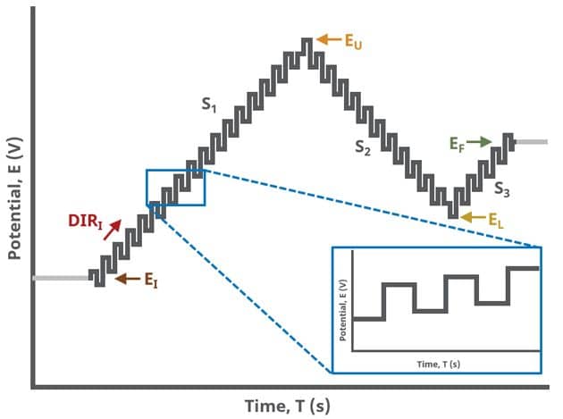
Figure 4. Square Wave Voltammetry (SWV) Three Segment Waveform

2Fundamental Equations

The following is a brief introduction to the theory of SWV. SWV was invented by Ramaley and Krause and thoroughly explained and further developed by the Osteryoungs. Refer to these references, including Bard and Faulkner's Electrochemical Methods for additional details on Square Wave Voltammetry. Cyclic Square Wave Voltammetry (CSWV), originally developed by Xinsheng and Guogang, and then revived by Helfrick and Bottomley, is covered in the literature also.

Consider a reaction $O + e^- \rightarrow R$ , where $O$ is reduced in a one-electron reaction to $R$ with formal potential, $E^{0}$ . An initial potential is applied to the electrode that is significantly more positive than $E^{0}$ . No significant faradaic current flows upon the application of forward pulse towards more positive values. Current is sampled at a specified point during the forward pulse.

The reverse pulse consists of stepping the potential of the working electrode to more negative values and the current is sampled near the end of the reverse pulse. The difference current is calculated by subtracting the reverse current from the forward current, given as

$i_d=i_{forward}-i_{reverse}$

As the potential of the working electrode approaches $E^{0}$ a faradaic current flows due to reduction of $O$ . Upon application of the reverse pulse, a faradaic current flows that effectively oxidizes the $R$ that was produced during the forward pulse. In other words, the rate of reduction slows compared to the forward step and an anodic current flows. Once the potential of the working electrode is sufficiently more negative of $E^{0}$ the current is diffusion-limited in both the forward and reverse pulse directions and the difference current is small.

The strength of SWV lies in its diagnostics, meaning that it is not typically used for quantitative analysis. It is possible; however, to calculate peak height using the equation

$\displaystyle {{\Delta}i_p = \frac{nFAD_O^{1/2}C_O^*}{{\pi}^{1/2}t_p^{1/2}}{\Delta}{\psi}}$

where $n$ is the number of electrons, $F$ is Faraday's Constant (96,485 C/mol), $A$ is the electrode area (cm²), $D_{0}$ is the diffusion coefficient of species $O$ (cm²/s), $C_O$ is the concentration of species $O$ (mol/cm³), $t_p$ is the experimental time scale $\displaystyle {1/2T_{SW,\; P}-T_{SW, \; W}}$ , and ${\Delta}{\psi}_p$ is a dimensionless peak Current parameter (see Table 1).

$n \Delta E_{A,\; SWV}/mV$	$n \Delta E_{I,\; SWV}/mV$
$n \Delta E_{A,\; SWV}/mV$	1	5	10	20
0^*	0.0053	0.0238	0.0437	0.0774
10	0.2376	0.2549	0.2726	0.2998
20	0.4531	0.4686	0.4845	0.5077
50	0.9098	0.9186	0.9281	0.9432
100	1.1619	1.1643	1.1675	1.1745

Table 1. Dimensionless Peak Current $({\psi}_p)$ vs. SWV Operating Parameters

The data in Table 1 were obtained in Electrochemical Methods. . *In Table 1, $n \Delta E_{I,\; SWV}/mV = 0$ corresponds to staircase voltammetry.

3Experimental Setup in AfterMath

To perform a square wave voltammetry experiment in AfterMath, choose Square Wave Voltammetry (SWV) from the Experiments menu (see Figure 5).

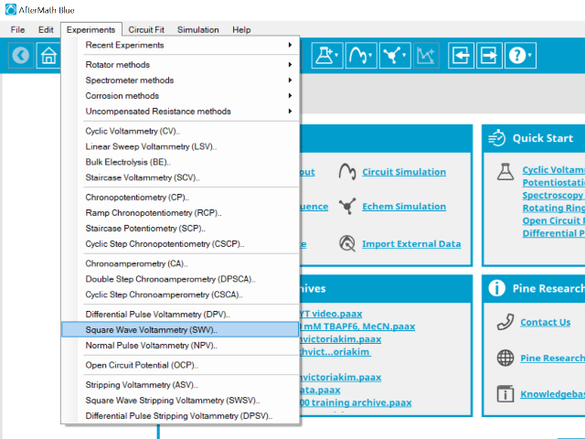
Figure 5. Square Wave Voltammetry (SWV) Experiment Menu Selection in AfterMath

Doing so creates an entry within the archive, called SWV Parameters. In the right pane of the AfterMath application, several tabs will be shown (see Figure 6).

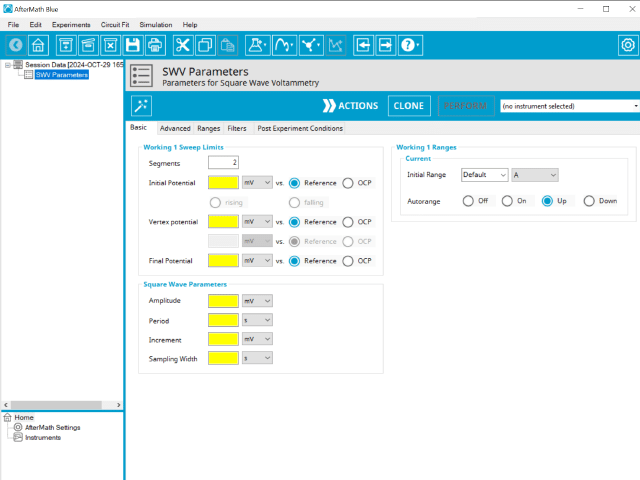
Figure 6. Square Wave Voltammetry (SWV) Experiment Basic Tab

As with many Aftermath methods, the experiment sequence is

Induction Period → Square Wave Sequence → Relaxation Period → Post-Experiment Idle Conditions

Continue reading for detailed information about the fields on each unique tab.

3.1Basic Tab

TIP: Click the AutoFill button ("I Feel Lucky" prior to May 2019) on the top bar in AfterMath to automatically fill all required parameters with reasonable starting values. While the values provided may not be appropriate for your specific system, they are reasonable parameters with which to start your experiment, especially if you are new to the method.

The basic tab contains fields for the fundamental parameters necessary to perform a SWV experiment. AfterMath shades fields with yellow when a required entry is blank and shades fields pink when the entry is invalid (see Figure 7).

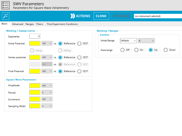
Figure 7. Square Wave Voltammetry (SWV) Basic tab in AfterMath

During the induction period, a set of initial conditions are applied to the electrochemical cell and the cell equilibrates at these conditions. Data are not collected during the induction period, nor are they shown on the plot during this period. Users will define induction period parameters on the Advanced Tab.

After the induction period, the potential of the working electrode is stepped through a series of increasing forward and reverse pulses from the Initial potential to the Final potential. The potential is incremented with each successive pulse according to the Pulse increment. In a typical experiment, Segments = 1 and there is a single series of pulses moving along the linear baseline from initial to final potential. Some may want to reverse the pulses (move in the opposite direction), accomplished by adjusting the number of segments to be > 1. By adjusting the number of segments, users can create variants of the DPV technique. Cyclic Square Wave Voltammetry consists of cycling (through a series of potential pulses also) the potential of the working electrode through a Vertex potential or between Upper potential and a Lower potential until reaching Final potential (Segments = 2 or 3).

The parameter settings for pulse-type experiments are often not as clear as with something more simple like Cyclic Voltammetry (a sweep method ). Refer to Figure 8 below when understanding each parameter of the DPV pulse. Further, clicking "AutoFill" ("I Feel Lucky" in older versions of AfterMath) provides reasonable starting parameters if you are unsure of typical values used in these experiments. Most often, research journal articles describe the SWV pulse sequence used, which can be replicated using AfterMath.

The experiment concludes with a relaxation period. During the relaxation period, a set of final conditions (specified on the Advanced tab) are applied to the electrochemical cell and the cell equilibrates at these conditions (set on the Advanced Tab). Data are not collected during the induction period, nor are they shown on the plot during this period.

At the end of the relaxation period, the post-experiment idle conditions are applied to the cell and the instrument returns to the idle state.

A plot of the typical experiment sequence, containing labels of the fields on the Basic tab, helps to illustrate the sequence of events in an SWV experiment (see Table 1 and Figure 8).

The table below lists the group and field names and symbols for each parameter associated with this experiment (see Table 1).

Group Name	Field Name	Symbol
Sweep (Sweep limits)	Segments	$S_N$
Sweep (Sweep limits)	Initial Potential	$E_I$
Sweep (Sweep limits)	Initial Direction	$DIR_I$
Sweep (Sweep limits)	Upper Potential	$E_U$
Sweep (Sweep limits)	Vertex Potential	$E_V$
Sweep (Sweep limits)	Lower Potential	$E_{LOW}$
Sweep (Sweep limits)	Final Potential	$E_F$
Square Wave	Amplitude	$E_{A, \;SWV}$
Square Wave	Period	$E_{P, \;SWV}$
Square Wave	Increment	$E_{E, \;SWV}$
Square Wave	Sampling width	$E_{W, \;SWV}$

Table 1. Basic Tab Group Names, Field Names, and Symbols.

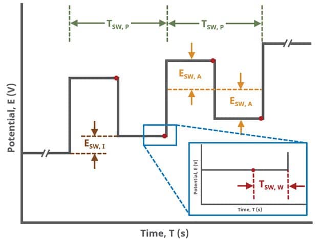
Figure 8. Square Wave Voltammetry (SWV) Pulse Sequence Detail

3.2Advanced Tab

The SWV Advanced tab contains groups for Induction Period, Relaxation Period, Pulse options, and iR Compensation (see Figure 9).

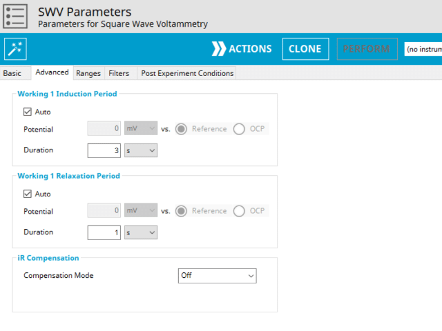
Figure 9. Square Wave Voltammetry (SWV) Experiment Advanced Tab in AfterMath

Induction Period is the first step in a SWV experiment if the Duration is >0 s. During the induction period, the specified current is applied to the cell for the specified duration. During this period, data are not collected. The Induction Period is believed to "calm" the cell prior to intentional perturbation (see Figure 10). More on Induction Period is found within the knowledgebase.

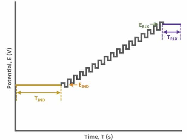
Relaxation Period is the last step in a SWV experiment if the Duration is >0 s. During the relaxation period, the specified current is applied to the cell for the specified duration. During this period, data are not collected. The Relaxation Period is believed to "calm" the cell after intentional perturbation (see Figure 10). More on Relaxation Period is found within the knowledgebase.

Figure 10. Square Wave Voltamemtry (SWV) Advanced Tab Fields

Detailed description of the iR Compensation Mode is provided elsewhere on the knowledgebase. This mode is used to correct for uncompensated resistance in the electrochemical cell.

Lastly, the iR Compensation group allows users to adjust the cell feedback to accommodate a known resistive drop between working and reference electrodes. Not all potentiostats from Pine Research support iR compensation. The WaveDriver series support iR compensation by positive feedback and current interrupt. The WaveDriver 100 and WaveDriver 200 support EIS-based iR compensation. The WaveNow series (including the WaveNano and WaveNow^XV ) and the CBP bipotentiostat do not support iR compensation of any type. More information about iR compensation, including understanding how it works and how to determine the resistance, consult the knowledgebase article on the topic.

3.3Ranges, Filters, and Post Experiment Conditions Tab

In nearly all cases, the groups of fields on the Ranges tab are already present on the Basic tab. The Ranges tab shows an Electrode Range group and depending on the experiment shows either, or both, current and potential ranges and the ability to select an autorange function. The fields on this tab are linked to the same fields on the Basic tab (for most experiments). Changing the values on either the Ranges tab or on the Basic tab changes the other set. In other words, the values selected for these fields will always be the same on the Ranges tab and on the Basic tab. More on ranges is found within the knowledgebase, as is for autorange.

The Filters tab provides access to potentiostat hardware filters, including stability, excitation, current response, and potential response filters. Pine Research recommends that users contact us for help in making changes to hardware filters. Advanced users may have an easier time changing the automatic settings on this tab. Filter settings fields are shown for WK1 (working electrode #1) as well as for WK2 (working electrode #2) regardless of the potentiostat connected to AfterMath.

By default, the potentiostat disconnects from the electrochemical cell at the end of an experiment. There are other options available for what these post-experiment conditions can be and are controlled by setting options on the Post Experiment Conditions tab.

4Sample Experiments

Below are the typical results for SWV (current difference) for the oxidation of a 1 mM solution of ferrocene n 0.1 M Bu₄NClO₄/CH₂CL₂ (see Figure 11). The specific parameters for this experiment are as follows:

Amplitude: 25 mV
Period: 10 ms
Increment: 2 mV
Sampling width: 1 ms

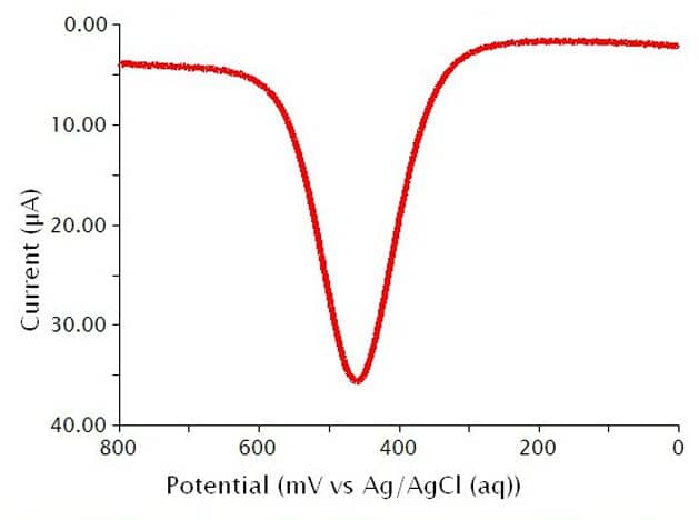
Figure 11. Square Wave Voltammogram (Difference Current) of a Ferrocene Solution

As mentioned previously, the default output plot from a SWV experiment is current difference (between forward and reverse pulses) vs. applied potential, as shown (see Figure 11). Under "Other Plots" there are square wave voltammograms for the forward pulse (see Figure 12) and reverse pulse (see Figure 13).

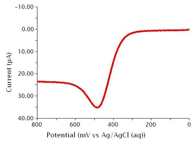
Figure 12. Square Wave Voltammogram (Forward Pulse Only) of a Ferrocene Solution

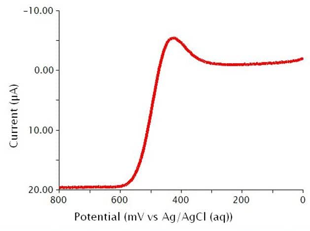
Figure 13. Square Wave Voltammogram (Reverse Pulse Only) of a Ferrocene Solution

Below is an example of Cyclic Square Wave Voltammetry, when Segments (S_N) > 1 (see Figure 14). Peak potentials are marked with a Crosshair tool to show that the anodic and cathodic peaks appear at nearly the same potential.

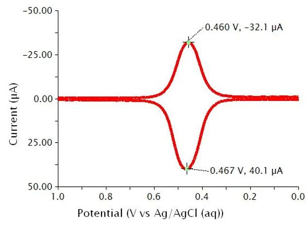
Figure 14. Cyclic Square Wave Voltammogram (Difference Current) for a Ferrocene Solution

5Example Applications

The first application uses SWV to monitor binding events associated with electrochemical sensors. White and Plaxco developed redox-tagged electrochemical sensors from electrode-bound oligonucleotides. Tuning the frequency of the voltammetric measurements allows the researchers to amplify both the unbound and target-bound signals, essentially, making an “On/Off” sensor.

In another example, Chakrabarti et. al used several electrochemical techniques, SWV among them, to monitor metal dissociation events. They combined RDE with anodic stripping voltammetry to distinguish between labile and nonlabile complexes in extremely low concentrations in aqueous solutions and in precipitation samples. The authors then showed that DPV, SCV, and SWV each provide similar dissociation constants; however, the sensitivity of SWV was two orders of magnitude higher than SCV. This is a nice example of how SWV compares with other electrochemical techniques.

How can we help? What do you want to learn? Search our knowledgebase.

Voltammetric Methods

Square Wave Voltammetry (SWV)

ARTICLE TAGS

CAPABLE POTENTIOSTATS

RELATED PAGES

AFTERMATH LINKS

Article Contents/Section Navigation

1Technique Overview

2Fundamental Equations

3Experimental Setup in AfterMath

3.1Basic Tab

3.2Advanced Tab

3.3Ranges, Filters, and Post Experiment Conditions Tab

4Sample Experiments

5Example Applications

6References

Questions? Find Answers.

Software

Applications

Theory

Product Specifications