


AfterMath EIS Data Import Procedure
Last Updated: 6/1/23 by Neil Spinner
1Abstract
This document describes how to import external electrochemical impedance spectroscopy (EIS) data into the Pine Research AfterMath Data Organizer software
 AfterMath Downloads
for analysis (e.g., circuit fitting, graphing). The procedure outlined herein is only valid on AfterMath versions 1.5.XXXX and later. Earlier versions of the software (i.e., 1.4.XXXX, 1.3.XXXX, or 1.2.XXXX) do not support EIS data generation, import, or analysis.
AfterMath Downloads
for analysis (e.g., circuit fitting, graphing). The procedure outlined herein is only valid on AfterMath versions 1.5.XXXX and later. Earlier versions of the software (i.e., 1.4.XXXX, 1.3.XXXX, or 1.2.XXXX) do not support EIS data generation, import, or analysis.
2Background
AfterMath software contains many powerful tools for analyzing electrochemical impedance spectroscopy (EIS) data. Tabulated EIS data collected using a competitor’s potentiostat, or otherwise generated and/or manually fabricated, may be imported into AfterMath quickly and easily. Once imported, analysis can be performed via a number of tools, most notably Circuit Fit or Kramers-Kronig. Imported and analyzed (fitted) data can then be saved, or exported if further analysis/manipulation by another software platform is required.
3Import Procedure
3.1Import External Data Option in File Menu
Click the "File" menu at the top left of the screen in AfterMath, then select the “Import External Data” option (see Figure 1). Alternately, the keystroke CTRL+I may be entered instead. A Multi-Column Data Import dialog box will open (see Figure 2). The default Data Specialization type for data import in AfterMath is “EIS” (which assumes frequency values in units of Hz); however, there are several other options in the dropdown menu, including “Mott-Schottky”, and both “EIS” or “Mott-Schottky” where the frequency may be in logarithmic units. For the scope of this document, only the default “EIS” option will be considered.
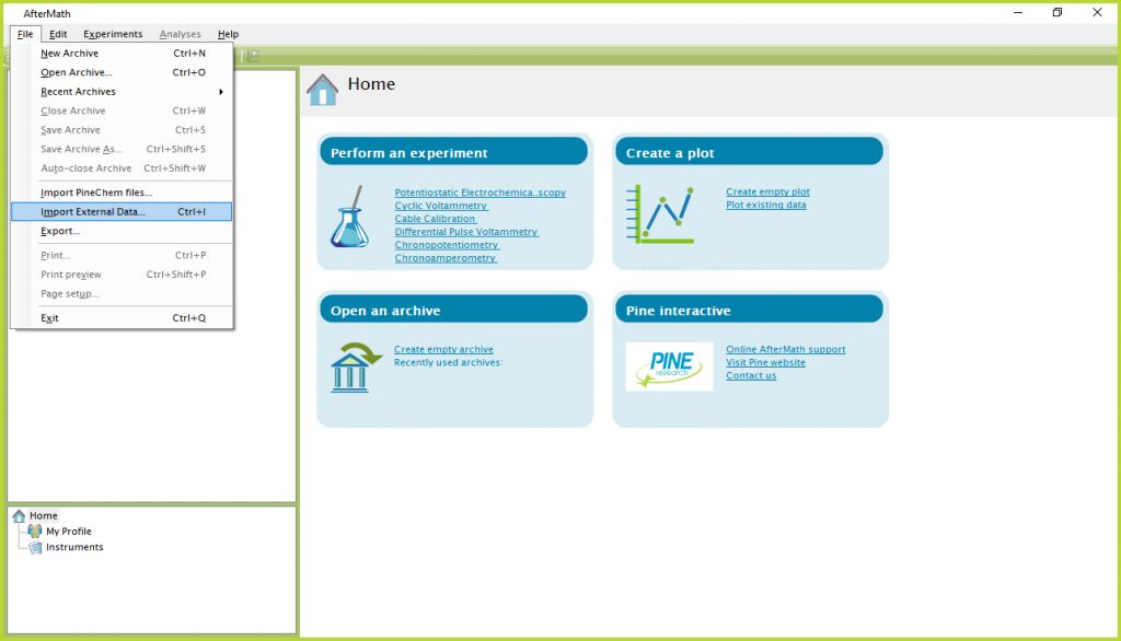
Figure 1. Location of Import External Data Option in AfterMath File Menu
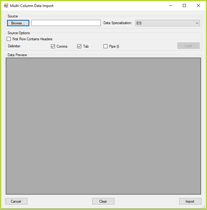
Figure 2. Multi-Column Data Import Dialog Box in AfterMath
3.1.1EIS Data Import via Copy/Paste
One option for importing EIS data into AfterMath is to simply copy and paste multiple columns of data directly into the dialog box. From the raw data file, copy the desired data columns onto the computer’s clipboard, then right-click in the dark gray section of the AfterMath Multi-Column Data Import dialog box and click “Paste” (see Figure 3).
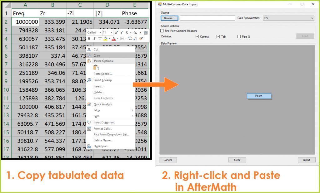
Figure 3. Copying and Pasting EIS Data into AfterMath
The data will appear in the dialog box and AfterMath automatically assigns variables to each column in order based on the typical logical order for EIS data: Frequency (in Hz), Real Impedance (Zr, in Ω), -Imaginary Impedance (-Zi, in Ω), Impedance Magnitude (|Z|, in Ω), then Phase Angle (Φ, in °) (see Figure 4). However, the drop-downs at the top of each column may be adjusted if the raw data columns do not agree with the default variable assignments.
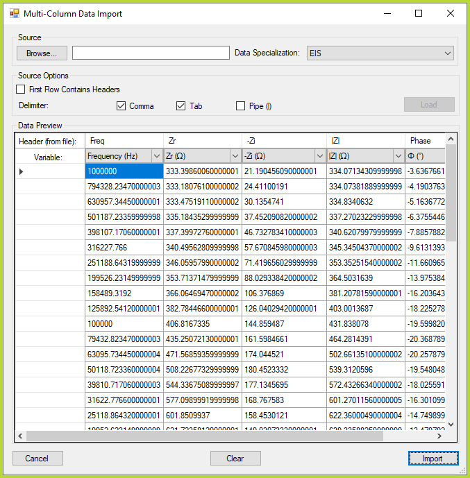
Figure 4. Pasted Five-Column EIS Data in AfterMath Import Dialog Box
The list of options for any data column in the dialog box drop-downs includes the five previously-mentioned variables, as well as non-negated Imaginary Impedance (Zi) and <Ignore>, which can be used if additional columns are pasted that do not contain EIS data or are not needed. AfterMath will appropriately skip over any data column with a drop-down set to <Ignore>.
Units for each variable, regardless of their column order in the dialog box, must be as defined above. For example, if the Phase Angle is in units of radians, the raw data must first be converted to degrees before attempting to import. Otherwise, the imported data in AfterMath will be incorrect.
It is not necessary to have all five columns of EIS data for a successful import. Only three columns of EIS data are strictly necessary, though the specific variables for those columns are important. For example, a user may import Frequency, Real Impedance, and Imaginary Impedance (either negated or non-negated), and AfterMath will automatically calculate the respective columns for Impedance Magnitude and Phase Angle. Conversely, a user may import Frequency, Impedance Magnitude, and Phase Angle, and AfterMath will automatically calculate the respective columns for Real Impedance and Imaginary Impedance. Any other combination of EIS variables is not currently supported by the Multi-Column Data Import feature in AfterMath.
Finally, once all necessary columns of EIS data have been pasted and variables appropriately assigned, click the “Import” button at the bottom right of the dialog box. A message will appear to indicate whether the import operation was successful or not. If the operation was successful, a new archive will appear in left tree structure of AfterMath with the imported data and automatically-generated Bode and Nyquist plots (see Figure 5). Additionally, the title of the imported data node will note the method of import. For example, for the previously-described copy/paste method, the title will read “Import from pasted data” (see Figure 5). If the data is imported via CSV file, the title will instead note the filename associated with the EIS data (see Section 3.1.2 for instructions on CSV file import).
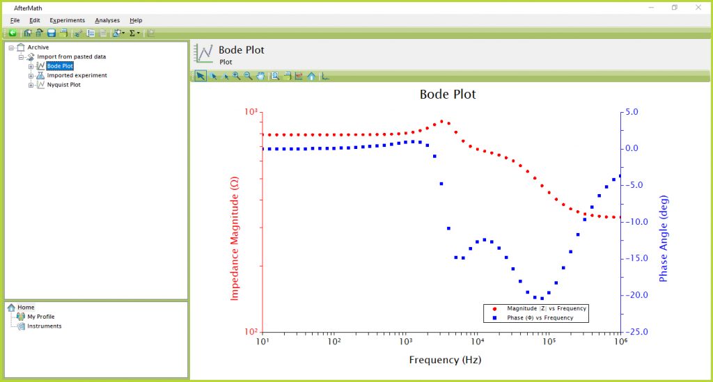
Figure 5. Successful Copy/Paste EIS Data Import in AfterMath
3.1.2EIS Data Import via CSV File
A second option for importing EIS data in AfterMath is via a Comma-Separated Values (CSV) file. Open the Multi-Column Data Import dialog box as previously-described (see Section 3.1 and Figure 1). Next, click the “Browse…” button, select the appropriate file from the file explorer window that appears, and click “Open”. The computer location of the selected file will populate in the bar next to the “Browse…” button. Click the “Load” button to temporarily view the data in the file. If the selected file is of the correct format and tabulated data exists, AfterMath will load the columns of data into the Multi-Column Data Import dialog box (see Figure 6).
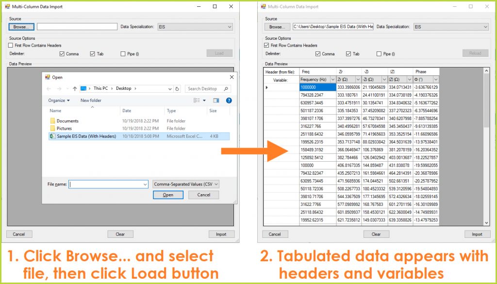
Figure 6. Importing EIS Data into AfterMath via CSV File
If the first row of values in the CSV file contains header text defining the column variables and/or units (typically for the user’s identification purposes), AfterMath will automatically detect the presence of text, rather than numerical entries, and the box next to “First Row Contains Headers” will be checked (see Figure 6). This setting will allow AfterMath to ignore the first row and begin importing where the numerical data begins. Further, if the first row does contain numerical values, the user may still toggle this check box to ignore the first row of data if desired.
If necessary, the user may click the “Clear” button at the bottom to start the import process over. Additionally, if any other incorrect setting was initially chosen, the button that previously showed “Load” will change to read “Reload” and the file can be loaded again to temporarily view the data with the proper import settings. These clearing and loading options may be toggled and repeated any number of times without consequence. Once the user is satisfied with the visible data in the Multi-Column Data Import dialog box and the selected variables for each column (see Section 3.1.1 for discussion of variables and proper units), click the “Import” button. Similarly to the previous copy/paste procedure, a message will indicate a successful data import, a new archive will appear in the left tree structure, and Bode and Nyquist plots will be automatically generated. The imported data node title will indicate the name of the imported CSV file (see Figure 7).
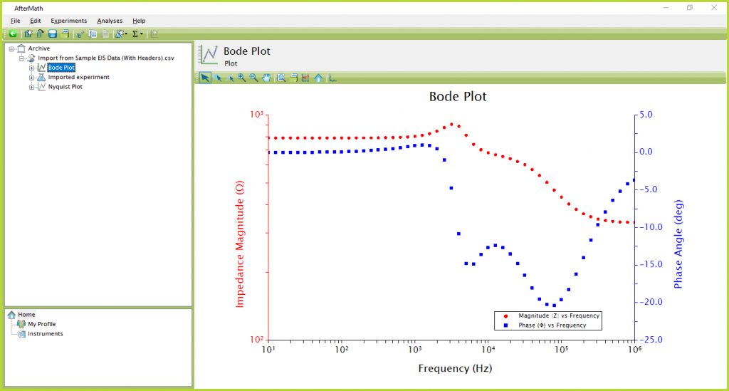
Figure 7. Successful CSV File EIS Data Import in AfterMath
4EU Customers: Fix for Comma/Period, Metric/U.S. Conventions
In the United States, numbers are written in the form "100,000.25" to represent for example "one hundred thousand point two five," or "one hundred thousand and 25/100ths." This is the convention that is default on PCs that are sold in the United States and also what AfterMath uses for reporting and processing numbers. However, in some countries (notably, much of Europe), the convention for displaying numbers reverses the use of periods and commas. In these cases, the same number above would possibly be displayed instead as "100.000,25"
When using AfterMath on a PC or in a region where this different period/comma is used, it may be necessary to modify the EIS data and/or adjust computer settings before importing into AfterMath. The first adjustment is to reverse the comma and period placement, which can typically be done when formatting as a *.CSV file using whichever program is being used to view and save the data. Alternatively, this task can be performed manually.
In some instances, even simply replacing the decimal place comma with a period alone can render the data in a form that can be imported into AfterMath. However, if the data is still not importing properly, or at all, the following steps may need to be taken:
Step 1: Open the control panel on the PC, and click "Change date, time, or number formats" under the heading "Clock and Region" (see Figure 8):
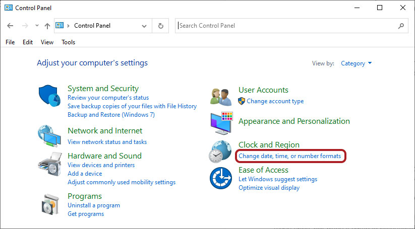
Figure 8. Control Panel on PC
Step 2: In the resulting window, click the "Additional settings..." button at the bottom (see Figure 9):
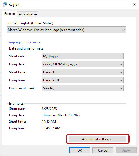
Figure 9. PC Number Formats
Step 3: In the next window, select "U.S." from the dropdown next to "Measurement system." The default will most likely be set to "Metric" (see Figure 10):
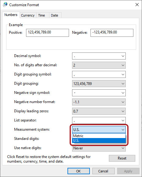
Figure 10. PC Measurement System