Knowledgebase

A set of results from a single individual experiment is usually stored as a data table in an archive. Data tables contain two-dimensional relationships which record how various signal levels change during an experiment. A simple set of results might include time-dependent measurements of several signals, such as voltage vs. time, temperature vs. time, or current vs. time.

Somewhat more complex relationships between signals might also be recorded. For example, the data table might also include a record of how one signal (i.e., an excitation signal) influences another signal (i.e., a response signal). Examples of these kind of relationships include current vs. voltage or temperature vs. heating coil current.

Still more complex relationships might involve a bit of post-experiment computation (post-processing) using the raw data. For example, it may be useful to record the ratio of a voltage signal to a current signal vs. time (perhaps to indicate how an electrical resistance changed during the experiment). Or, it might be of interest to view how the current signal changes versus the square root of time (perhaps to elucidate how diffusion influences the measured current).

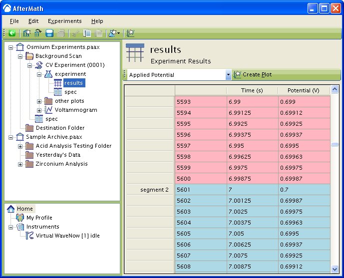
Regardless of the complexity of a signal relationship or how it is computed, this kind of two dimensional data is generally recorded as a set of ordered pairs, most often appearing as two columns of numeric data as shown in the figure below.

The data visible in the example (above) is a portion of a triangle waveform describing a voltage that was applied to an electrode during a voltammetry experiment. The voltage was recorded every 1.25 milliseconds, and the portion of data shown was measured about seven seconds into the experiment. Using the scroll bar along the side of the data table, it is possible to view data acquired at earlier or later points in the experiment.

The background shading in a data table often indicates additional information about a particular segment of the data. The default shading color is gray, but alternating pink and blue shading is often used to indicate the boundary between adjacent segments. In the example above, the pink shading indicates data recorded during the first segment of the triangle wave where the voltage signal is increasing versus time. The blue shading indicates the second segment of the triangle wave where the the voltage begins to decrease with time. In addition an entry is placed in the first column of the table to indicate the start of the second segment.

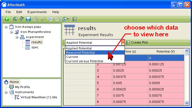
Many instruments produce more than one signal of interest during a given experiment. AfterMath groups all of the related signals from an experiment together into one data table in the archive. When you view a data table which contains more than one signal, it appears as shown below. There is a drop down list at the top of the display area which allows you to choose which signal relationship is displayed. In the example below, there are four different signal relationships which can be viewed.

Scientists typically prefer to view signal measurements as traces on a plot rather than tables of numbers. If you would like to view a signal on a plot, simply click on the “Create Plot” button near the top of the table.

More details about this option are found later in this manual (click here).