


Potentiostat Diagnostic Tests
Back to Potentiostat Diagnostic Tests Back to Applications Back to Knowledgebase HomeWaveDriver Shorted Lead EIS Test
Last Updated: 1/5/23 by Alex Peroff
1WaveDriver Shorted Lead EIS Test
A “shorted lead” test explores the absolute lower load measurement limit for EIS measurements across a range of frequencies. Measurements made at these extreme limits fall well outside the outermost region of an Accuracy Contour Plot.
 EIS Accuracy Contour Plot
The shorted lead test is a quick diagnostic test, and the results of the test should never be interpreted as a measurement of instrument accuracy.
EIS Accuracy Contour Plot
The shorted lead test is a quick diagnostic test, and the results of the test should never be interpreted as a measurement of instrument accuracy.
This test is performed during the system testing of a Pine Research WaveDriver potentiostat (WaveDriver 200
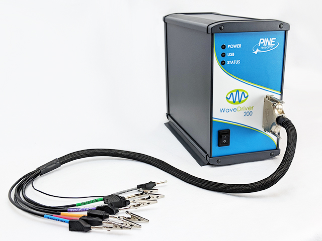 WaveDriver 200 EIS Bipotentiostat/Galvanostat
and WaveDriver 100
WaveDriver 200 EIS Bipotentiostat/Galvanostat
and WaveDriver 100
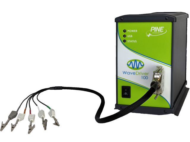 WaveDriver 100 EIS Potentiostat/Galvanostat
models).
WaveDriver 100 EIS Potentiostat/Galvanostat
models).
WaveDriver 200 EIS Bipotentiostat/Galvanostat
and WaveDriver 100
WaveDriver 100 EIS Potentiostat/Galvanostat
models). 1.1Low Inductance Cell Cable Configuration
When measuring a low impedance load (<10 Ω), it is good practice to configure and route the cell cable in a manner that minimizes the inductance of the cell cable. Braiding the sense lines together and separately braiding the drive lines together (see Figure 1) minimizes the contribution of the cell cable inductance to the overall load measured by the instrument. Inductive interference from the cell cable is further minimized by maintaining as much separation between the drive lines and sense lines as possible.
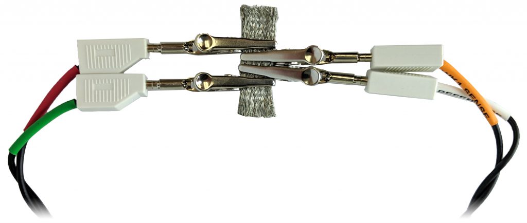
Figure 1. Braided Cell Cable Configuration for Low Inductance Load Measurement
The “load” used in a shorted lead test is a conductive material with very low impedance (typically a short length of copper wire or a conductive metal mesh). The load is essentially a “short circuit” with an extremely small resistance (≪1 mΩ), so it is very important to use the low inductance (braided) cell cable configuration during a shorted lead test. In the example shown (see Figure 1), a conductive metal mesh is used as the load. Both of the sense lines – WHITE (reference) and ORANGE (K1 sense) – are physically braided together and clipped side-by-side to the mesh.
Similarly, both of the drive lines – GREEN (counter) and RED (K1 drive) – are physically braided together, routed as far away from the sense lines as possible, and brought to the opposite side of the load. The RED lead (K1 drive) is clipped to the wire as close to the ORANGE lead (K1 sense) as possible. The GREEN lead (counter) is clipped to the wire as close to the WHITE lead (reference) as possible.
As is always good practice in any EIS experiment, the cables and the load are placed inside a metal Faraday cage (see Figure 2). The instrument chassis is connected to the Faraday cage by connecting the GRAY lead on the cell cable to any convenient connection point on the metal Faraday cage.
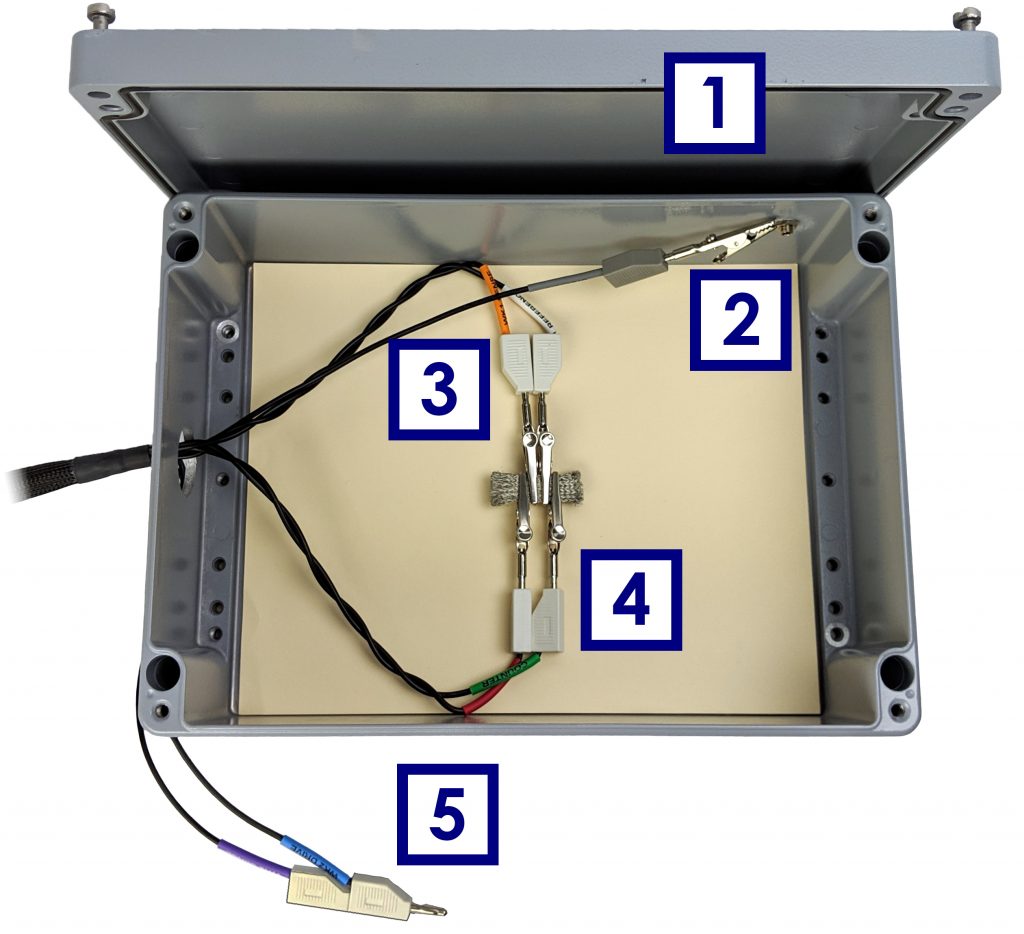
| 1 | The metal Faraday cage should have a lid (shown here in the open position) |
| 2 | The GRAY banana plug should be electrically connected to the metal Faraday cage |
| 3 | The WHITE/ORANGE braided sense lines should connect to the load on one side |
| 4 | The GREEN/RED braided drive lines should connect to the load from the other side |
| 5 | The BLUE/PURPLE lead pair should be placed outside the Faraday cage. NOTE: This lead pair is only present on the WaveDriver 200 cell cable. These leads do not appear on the WaveDriver 100 cell cable. |
Figure 2. Proper Cable Arrangement for an Open Lead EIS Measurement
1.2Create a Galvanostatic EIS Experiment (EIS-GAL)
Choose the Galvanostatic Electrochemical Impedance Spectroscopy (EIS-GAL) option from the Impedance Spectroscopy sub-menu in the AfterMath Experiments menu. A new EIS-GAL specification will be created and placed into a new archive. Configure the parameters as shown (see Figure 3).
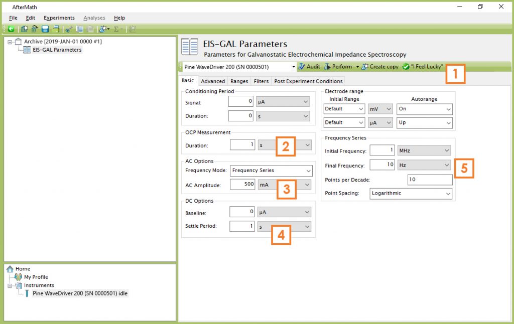
| 1 | Click on the “I Feel Lucky” button. Note that default parameters for OCP Measurement Duration, AC Amplitude, DC Baseline, and Frequency Series appear automatically. |
| 2 | Set the OCP Measurement Duration to 1 s |
| 3 | Set the AC Amplitude to 500 mA |
| 4 | Set the DC Options Settle Period to 1 s |
| 5 | Set the Final Frequency to 10 Hz |
Figure 3. Parameters used for a Shorted Lead EIS Test
1.3Audit Experimental Parameters
Choose the WaveDriver in the drop-down menu (see Figure 4, to the left of the “Audit” button). Press the “Audit” button to check the parameters. AfterMath will perform a quick audit of the parameter values to ensure that all required parameters have been specified and are within allowed ranges.
1.4Initiate the Experiment
Click on the “Perform” button to initiate the EIS-GAL Shorted Lead experiment. The “Perform” button is located to the right of the “Audit” button (see Figure 4).
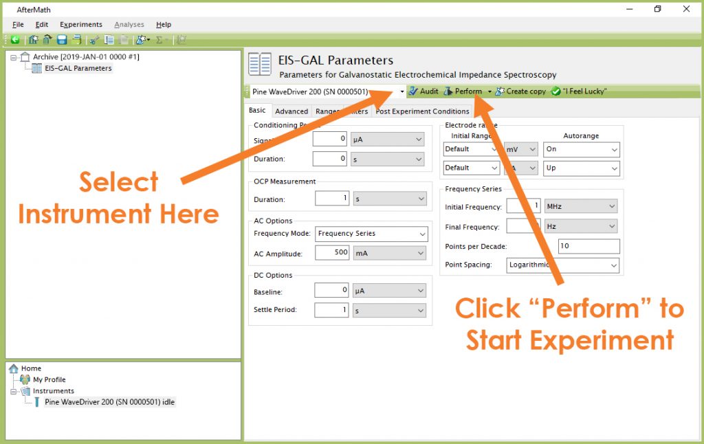
Figure 4. Location of Instrument Selection Menu and Perform Button (EIS-GAL)
1.5Monitor Experimental Progress
Monitor the progress of the EIS-GAL Shorted Lead experiment in AfterMath by observing the real time plot and the progress bar (see Figure 5). The default live display shows Lissajous plots, but Bode or Nyquist plots can also be observed in real time if desired.
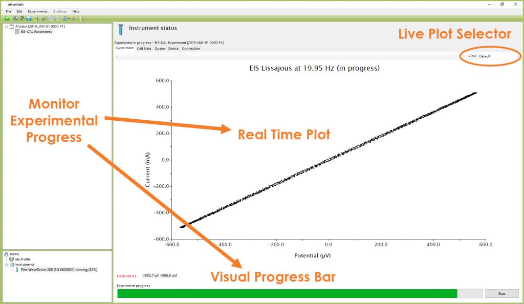
Figure 5. Monitoring the Progress of the EIS-GAL Shorted Lead Experiment
1.6Review the Results
When the experiment has finished, the results of the shorted lead test are placed in a folder within the archive. Examination of the Bode plot (see Figure 6) at lower frequencies (≤50 Hz) shows how the load nearly behaves like an ideal resistor (i.e., the phase angle is nearly zero) with a very small resistance (~250 μΩ).
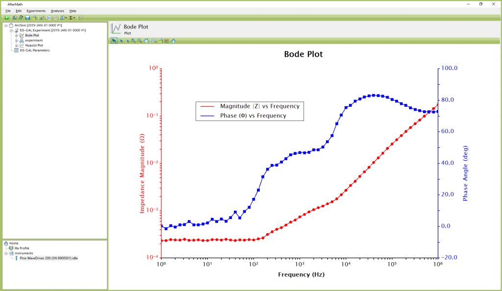
Figure 6. Bode Plot for a Typical Shorted Lead EIS Test
This small resistance represents the lowest possible load measurement that can be made with the instrument, and it is related to the sum of the resistance of the cell cable leads, the contact resistance of the alligator clips with the load, and the small resistance of the load itself. This minimal residual resistance falls well below the range of impedance loads normally encountered in routine EIS experiments, and it also falls below the lower limit of the Accuracy Contour Plot.
Product Specifications
EIS Accuracy Contour Plot Nevertheless, the user may wish to measure this residual resistance and subtract it from EIS results in those cases where the load being studied is quite small (≤20 mΩ).
EIS Accuracy Contour Plot Nevertheless, the user may wish to measure this residual resistance and subtract it from EIS results in those cases where the load being studied is quite small (≤20 mΩ).
As the frequency increases, the Bode plot shows a gradual increase in the observed load as the phase angle increases toward ninety degrees (+90°). The inductive properties of the cell cable begin to dominate at higher frequencies, imposing an extreme limit (e.g., “the inductive limit”) beyond which the instrument cannot make a measurement. Again, this extreme limit falls well outside the accuracy limits on an Accuracy Contour Plot.