Cyclic Voltammetry (CV)

Last Updated: 1/10/23 by Alex Peroff

ARTICLE TAGS

current vs. potential,
CV,
Cyclic Voltammetry,
AfterMath CV

RELATED PRODUCTS

AFTERMATH LINKS

Linear Sweep Voltammetry (LSV)

Article Contents/Section Navigation

1Technique Overview

Cyclic Voltammetry (CV) is one of the most ubiquitous electrochemical methods used today. There are many variations of CV including Rotating Disk Voltammetry (RDE), Rotating Ring-Disk Voltammetry (RRDE), and Rotating Cylinder Electrochemistry (RCE). In CV, working electrode potential is swept linearly between final and initial values, possible with intermediate upper, lower, and/or vertex values, and current is measured as a function of time. The most common output from a CV experiment is current vs. potential, called a voltammogram.

At its most basic level, CV sweeps potential vs. reference electrode in forward and reverse directions, often through the electroactive species' E⁰, which allows for the investigation of the resulting electrochemical species generated at the electrode surface. CV provides both qualitative and quantitative information about electrochemical systems and has become well-established as a fast and reliable characterization tool. CV is often used to study the kinetics of electron transfer reactions, including catalysis, and has been expanded for use in organic and inorganic synthesis, sensor and biological system evaluation, and fundamental physical mechanics of electron transfer reactions, such as reversibility, formal potentials, and diffusion coefficient determination. While CV may have been developed by a smaller group of physical electrochemists, the gain in popularity of the technique finds users from inorganic chemistry, materials chemistry, and even biological chemistry.

In the simplest case, when Segments (S_N) = 1, potential is swept linearly from an initial to final potential, sampling current at specified intervals (see Figure 1).

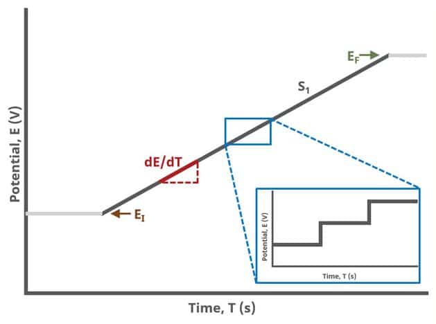
Figure 1. Cyclic Voltammetry (CV) One Segment Waveform

When Segments (S_N) = 2, potential is swept linearly from an initial to vertex potential and back to final potential, sampling current at specified intervals (see Figure 2).

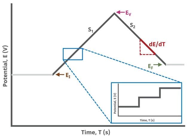
Figure 2. Cyclic Voltammetry (CV) Two Segment Waveform

When Segments (S_N) ≥ 3, potential is swept linearly from an initial to final potential with two additional turning points called upper and lower potential, sampling current at specified intervals (see Figure 3). In this case, the most advanced waveform can be designed.

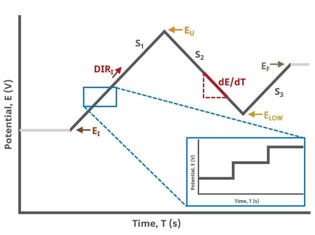
Cyclic Voltammetry (CV0 Three Segment Waveform

Figure 3. Cyclic Voltammetry (CV) Three Segment Waveform

Modern Pine Research potentiostats have digital waveform generators on board. This means that linear sweeps are approximated by a series of small stair steps, whose step size is defined by the 16-bit resolution Analog-to-Digital converter (ADC) on the circuit board and current/potential range selected. For example, on the WaveDriver 100, , the current step resolution on the ±100 nA range is

$\displaystyle \frac{200 \: \text{nA}}{2^{16}}=3.1 \: \text{pA}$

Appropriate current and/or potential filters are automatically employed to "smooth" the jagged edges of this step sequence, enhancing the linearity of the sweep, but can be controlled by the user on the Filters tab of any experiment.

2Fundamental Equations

A brief summary of the theory of cyclic voltammetry will be covered here. Randles and Ševčík contributed to the development of the theory for cyclic voltammetry; however, credit for the modern treatment and notation is attributed to Nicholson and Shain. Additionally, Bard and Faulkner provide a nice summary and description of cyclic voltammetry as do Kissinger and Heinemann.

Consider a reaction,

$O+e^- \rightleftharpoons R$

with a formal potential $E^{\circ}$ . If a potential sweep is started sufficiently more positive than $E^{\circ}$ and swept negatively, a non-faradaic current will initially flow. As the potential of the electrode approaches $E^{\circ}$ , $O$ starts reducing to $R$ , which creates a concentration gradient leading to an increased flux (mass transfer) to the surface of the electrode. As $E$ passes $E^{\circ}$ , the concentration of $O$ at the surface of the electrode is nearly zero and mass transfer reaches its maximum. The current begins to tail as the potential is swept to the vertex potential, upon which the sweep is reversed.

The concentration of $R$ at the surface of the electrode is now high and oxidation proceeds once $E$ begins to approach $E^{\circ}$ . An inverse of the process described above arises and results in a similarly shaped, but inverted, i-E curve. Ideally, the peak-to-peak separation for the reduction and oxidation waves is 59 mV for a one-electron electrochemically reversible process. Additionally, the peak height $i_p$ in amperes (A) is be described by the Randles-Ševčík equation,

$\displaystyle i_p=0.4463NFAC{\left(\frac{nF\upsilon D}{RT}\right)}^{1/2}$

where $n$ is the number of electrons, $F$ is Faraday’s Constant (96,485 C/mol), $A$ is the electrode area, $D$ is the diffusion coefficient, $C$ is the concentration, $R$ is the universal gas constant (8.314 J/mol⋅K), $T$ is the absolute temperature (K) and ${\upsilon}$ is the sweep rate. At 25°C, the equation simplifies to

$\displaystyle i_p=2.69\times10^5n^{3/2}AD^{1/2}C{\upsilon}^1/2$

As a general approximation,

$i_p\approx 200 \: \mu\text{A}/\text{cm}^2 \:\text{area/mM} \; (n=1,\: \upsilon=0.1 \: \text{V/s})$

3Experimental Setup in AfterMath

To perform a cyclic voltammetry experiment in AfterMath, choose Cyclic Voltammetry (CV) from the Experiments menu (see Figure 4).

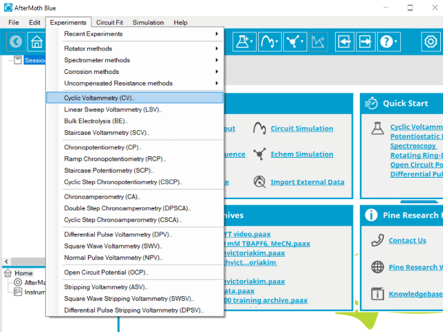
Figure 4. Cyclic Voltammetry (CV) Experiment Menu Selection in AfterMath

Doing so creates an entry within the archive, called CV Parameters. In the right pane of the AfterMath application, several tabs will be shown (see Figure 5).

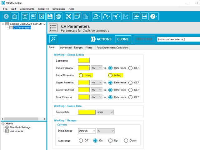
Figure 5. Cyclic Voltammetry (CV) Experiment in AfterMath

As with many Aftermath methods, the experiment sequence is

Induction Period → Sweep → Relaxation Period → Post-Experiment Idle Conditions

Like many methods, the Induction and Relaxation Periods are on the Advanced Tab. The parameters for a CV experiment are fairly simple compared to other methods in AfterMath.

In general, enter minimum required parameters on the Basic tab and press "Perform" to run an experiment. AfterMath will perform a quick audit of the parameters you entered to ensure their validity and appropriateness for the chosen instrument, followed by the initiation of the experiment. In some cases, users may desire to adjust additional settings such as filters, post- experiment conditions, and post-experiment processing before clicking the "Perform" button. Continue reading for detailed information about the fields on each unique tab.

3.1Basic Tab

TIP: Click the AutoFill button ("I Feel Lucky" prior to May 2019) on the top bar in AfterMath to automatically fill all required parameters with reasonable starting values. While the values provided may not be appropriate for your specific system, they are reasonable parameters with which to start your experiment, especially if you are new to the method.

The basic tab contains fields for the fundamental parameters necessary to perform a CV experiment. AfterMath shades fields with yellow when a required entry is blank and shades fields pink when the entry is invalid (see Figure 6).

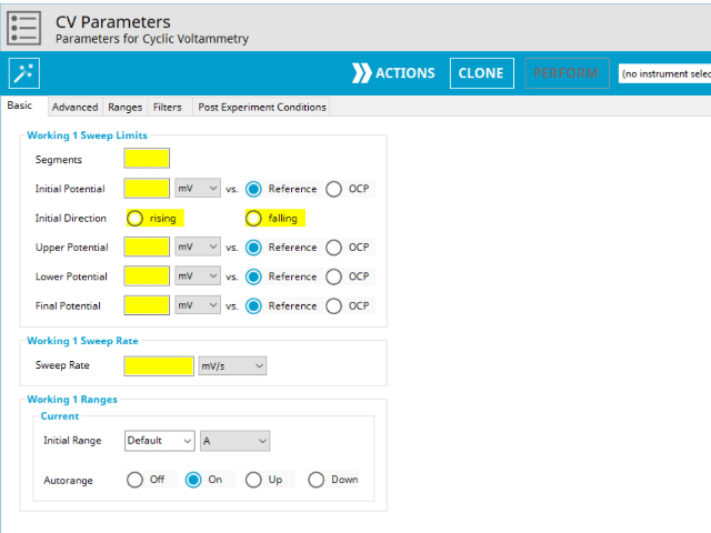
Figure 6. Cyclic Voltammetry (CV) Experiment Basic Tab in AfterMath

During the induction period, a set of initial conditions are applied to the electrochemical cell and the cell equilibrates at these conditions (set on the Advanced Tab). Data are not collected during the induction period, nor are they shown on the plot during this period.

After the induction period, the potential applied to the working electrode is swept to the next specified value (based on segments) for the duration of the experiment, which is called the sweep period. The potentiostatic circuit of the instrument maintains control over increasing potential while simultaneously measuring the current at the working electrode relative to the reference electrode. During the sweep segments, potential and current at the working electrode are recorded at regular intervals as specified on the Advanced Tab.

The experiment concludes with a relaxation period. During the relaxation period, a set of final conditions (specified on the Advanced tab) are applied to the electrochemical cell and the cell equilibrates at these conditions (set on the Advanced Tab). Data are not collected during the induction period, nor are they shown on the plot during this period.

A plot of the typical experiment sequence, containing labels of the fields on the Basic tab, helps to illustrate the sequence of events in a CV experiment (see Table 1 and Figure 7).

The table below lists the group and field names and symbol for each parameter associated with this experiment (see Table 1).

Group Name	Field Name	Symbol
Sweep	Segments	$S_N$
Sweep	Initial Potential	$E_I$
Sweep	Initial Direction	$DIR_I$
Sweep	Upper Potential	$E_U$
Sweep	Vertex Potential	$E_V$
Sweep	Lower Potential	$E_{LOW}$
Sweep	Final Potential	$E_F$
Sweep	Sweep Rate	$dE/dT$

Table 1. Basic Tab Group Names, Field Names, and Symbols.

Figure 7. Cyclic Voltammetry (CV) Three Segment Waveform Field Diagram

CV is one of several methods in AfterMath where users can specify the number of Segments (S_N) that will be used in the waveform. As described in Section 1 above, there are different fields used based on the number entered into the Segments field. When S_N ≥ 2, Vertex Potential field is shown on the Basic Tab. When S_N ≥ 3, Vertex Potential field is replaced with Upper Potential and Lower Potential fields on the Basic tab.

The Electrode Range group on the Basic Tab is used to specify the expected potential and/or current range to use on the experiment. For CV, current is the measured valued and as such, users can select the most appropriate current range from the dropdown menu. The most appropriate range is the one that completely includes the expected current spread across the entire experiment, but it not significantly greater. Note that the selection chooses the initial range. If Autorange is not Off, then as data are collected, AfterMath will choose the most appropriate range as needed. If Autorange is Off, and the initial range is too small, then current may go off scale and the results will be truncated. If the initial current range is too large, and Autorange is Off, then the data may have a noisy, choppy, or quantized appearance. More on the topic of Electrode Range is provided elsewhere in the knowledgebase.

At the end of the relaxation period, the post-experiment idle conditions are applied to the cell, and the instrument returns to the idle state. The default plot generated from the data is measured current vs. potential, called a voltammogram.

3.2Advanced Tab

The CV Advanced tab contains groups for Induction Period, Relaxation Period, iR Compensation, and Sampling (see Figure 8).

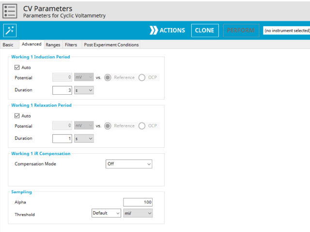
Figure 8. Cyclic Voltammetry (CV) Experiment Advanced Tab in AfterMath

Induction Period is the first step in a CV experiment if the Duration is >0 s. During the induction period, the specified current is applied to the cell for the specified duration. During this period, data are not collected. The Induction Period is believed to "calm" the cell prior to intentional perturbation. More on Induction Period is found within the knowledgebase.

Relaxation Period is the last step in a CV experiment if the Duration is >0 s. During the relaxation period, the specified current is applied to the cell for the specified duration. During this period, data are not collected. The Relaxation Period is believed to "calm" the cell after intentional perturbation. More on Relaxation Period is found within the knowledgebase.

Detailed description of the iR Compensation Mode is provided elsewhere on the knowledgebase. This mode is used to correct for uncompensated resistance in the electrochemical cell.

The Sampling group defines the potential sampling rate for the experiment There are two parameters in this group, Alpha and Threshold. As mentioned previously, digital instruments (such as the WaveNow and WaveDriver series potentiostats) approximate a linear sweep with a series of tiny steps.

As shown, alpha is the total time after each small step, from 0% to 100% and the value of alpha defines the time at which a sample is measured (see Figure 9). If $\alpha=0$ , current is measured immediately after the small step. If $\alpha=100$ then current is measured just before the next small step. In general, it is recommended to measure sweep experiments at $\alpha=100$ , which is the default setting.

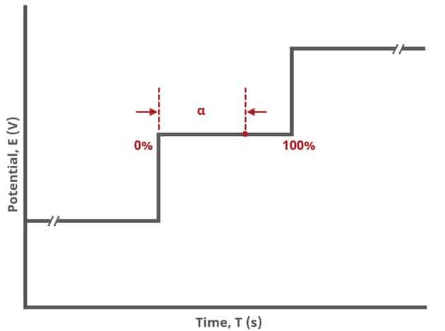
Figure 9. Potentiostatic Approximation of a Linear Sweep (Micro View)

Threshold defines the frequency of sampling. There are two options from the dropdown which are "Default" and "None." Additionally, a specific current interval can be added by typing a numeric value into the dropdown box and selecting the appropriate units. Briefly, the options can be described as follows:

Default. This setting will use the default settings, which are 5 mV for potentiostatic experiments and 1 µA for galvanostatic experiments.
None. This setting will enable the collection of the maximum number of data points possible. The value is not easily known, as is a combination of the sweep rate and sweep limits. Choose this option to collect the maximum number of data points that the hardware can acquire.
Manual entry. In this case, type an integer value into the dropdown menu and select the appropriate units in the next dropdown menu. For example, a user may only wish to collect a data point every 20 mV, in which case these are entered into the fields.

NOTE: Not all threshold values, manually entered, will be allowed. The software will use the value provided and match as closely to it as possible. The actual sampling rate may be higher, exact, or lower than the value entered. Presently, AfterMath will not inform you of the threshold value actually possible, but it can be inferred after the completion of the experiment and viewing the time-based data stream, where the threshold can be calculated as the time difference between data points.

NOTE: Archive file size increases as the threshold decreases. In other words, a smaller threshold means more data will be collected per experiment whereas a larger threshold means fewer data will be collected per experiment. For long term experiments, Pine Research recommends the default threshold, unless users require a finer level of detail per sweep.

Lastly, the iR Compensation group allows users to adjust the cell feedback to accommodate a known resistive drop between working and reference electrodes. Not all potentiostats from Pine Research support iR compensation. The WaveDriver series support iR compensation by positive feedback and current interrupt. The WaveDriver 100 and WaveDriver 200 support EIS-based iR compensation. The WaveNow series (including the WaveNano and WaveNow^XV WaveNowXV Potentiostat/Galvanostat Basic Bundle ) and the CBP bipotentiostat do not support iR compensation of any type. More information about iR compensation, including understanding how it works and how to determine the resistance, consult the knowledgebase article on the topic.

3.3Ranges, Filters, and Post Experiment Conditions Tab

In nearly all cases, the groups of fields on the Ranges tab are already present on the Basic tab. The Ranges tab shows an Electrode Range group and depending on the experiment shows either, or both, current and potential ranges and the ability to select an autorange function. The fields on this tab are linked to the same fields on the Basic tab (for most experiments). Changing the values on either the Ranges tab or on the Basic tab changes the other set. In other words, the values selected for these fields will always be the same on the Ranges tab and on the Basic tab. More on ranges is found within the knowledgebase, as is for autorange.

The Filters tab provides access to potentiostat hardware filters, including stability, excitation, current response, and potential response filters. Pine Research recommends that users contact us for help in making changes to hardware filters. Advanced users may have an easier time changing the automatic settings on this tab. Filter settings fields are shown for WK1 (working electrode #1) as well as for WK2 (working electrode #2) regardless of the potentiostat connected to AfterMath. More information on filters is available elsewhere on the knowledgebase.

By default, the potentiostat disconnects from the electrochemical cell at the end of an experiment. There are other options available for what these post-experiment conditions can be and are controlled by setting options on the Post Experiment Conditions tab.

4Sample Experiment

Peak currents from cyclic voltammograms are often studied and measured for their quantitative information. As predicted by the equation above, peak current increases with the sweep rate (see Figure 10). Here, 1 mM K₃Fe(CN)₆ in 0.1 M KCl was studied with CV at various scan rates = 20, 50, 100, 250, and 500 mV/s for red, gold, green, blue, and black traces, respectively. When these peak current values are plotted vs. 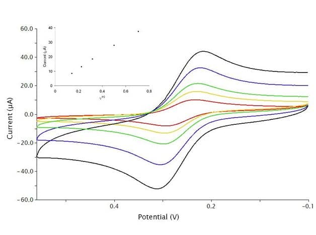$\upsilon^{1/2}$ the result is a straight line (see Figure 10, inset), whose slope can be used to find diffusion coefficient as shown below.

Figure 10. Cyclic Voltammetry (CV) Scan Rate Study of Ferricyanide

From above, the simplified Randles-Ševčík equation is

$\displaystyle i_p=2.69\times10^5n^{3/2}AD^{1/2}C{\upsilon}^1/2$

Rearrangement of the equation to linear form, with constant $C$ yields

$\displaystyle i_p=(2.69\times10^5n^{3/2}AD^{1/2}C){\upsilon}^{1/2}+0$

where the slope, from the inset plot in Figure 10, is equal to

$m=2.69\times10^5n^{3/2}AD^{1/2}C$

when $C$ is constant, the diffusion coefficient (in cm²/s) is calculated from the slope

$D=\dfrac{m}{2.69\times10^5n^{3/2}AC}$

Instead, one can conduct a similar study in which the concentration of the redox couple is changed while holding the sweep rate constant. In a similar fashion as described above, the diffusion coefficient can be calculated from the slope of the line from a plot of $i_p \:\text{vs.}\:C$ .

5Example Applications

Cyclic Voltammetry is versatile and a very well-known and used electrochemical method. In fact, CV is often the only thing non-electrochemists know about electrochemistry. Due to the avian shape of the classical, reversible cyclic voltammogram, many refer to them as ducks. . Many researchers from other research areas and disciplines have made CV part of their central research science, including traditionally inorganic chemists and materials scientists. There are too many excellent examples of CV in the literature and textbooks to enumerate a list of applications here. Instead, we only focus on two interesting applications from the literature.

The first example shows how CV can be used to calculate electron transfer rate constants. The theory for calculating electron transfer rate constants from cyclic voltammetry was originally developed by Nicholson but the example here is from more recent work by Weber and Creager. Ferrocene was irreversibly adsorbed in the form of a self-assembled monolayer to an Au surface using a long-chain alkylthiol. Varying the sweep rates gave increasingly larger $E_{peak} - E^0$ values ( $\eta$ , overpotential), with $E_{peak}$ being the oxidation or reduction peak and $E^0$ being the formal potential for ferrocene in this system. Rate constants were then calculated from these overpotentials. The authors compared the experimentally obtained voltammograms to theoretically calculated voltammograms thereby obtaining reorganization energies.

In the second example, Duah-Williams and Hawkridge used cyclic voltammetry to study the temperature dependence of the kinetics of CN^- dissociation from the cyanomyoglobin complex (Mb(II)CN ). By comparing the experimentally obtained cyclic voltammograms to theoretically calculated cyclic voltammograms, they were able to estimate the dissociation rate, k_f , by varying the sweep rate and monitoring the disappearance of an oxidation wave associated with Mb(II)CN, as CN^- dissociated. This research illustrates how CV can be used to elucidate details such as dissociation constant, which has traditionally been measured using more cumbersome NMR.

How can we help? What do you want to learn? Search our knowledgebase.

Voltammetric Methods

Cyclic Voltammetry (CV)

ARTICLE TAGS

RELATED PRODUCTS

RELATED PAGES

AFTERMATH LINKS

Article Contents/Section Navigation

1Technique Overview

2Fundamental Equations

3Experimental Setup in AfterMath

3.1Basic Tab

3.2Advanced Tab

3.3Ranges, Filters, and Post Experiment Conditions Tab

4Sample Experiment

5Example Applications

6References

Questions? Find Answers.

Software

Applications

Theory

Product Specifications