


Generate Tafel Plots in AfterMath from CV or LSV Data
Last Updated: 5/7/19 by Tim Paschkewitz
1Abstract
AfterMath can be used to convert cyclic voltammetry (CV)
 Cyclic Voltammetry (CV)
and linear sweep voltammetry (LSV)
Linear Sweep Voltammetry (LSV)
data from typical current vs. potential plots to Tafel representations, such as potential vs. log current density. The steps to perform this transformation are documented here, but the process is still manual at present.
Cyclic Voltammetry (CV)
and linear sweep voltammetry (LSV)
Linear Sweep Voltammetry (LSV)
data from typical current vs. potential plots to Tafel representations, such as potential vs. log current density. The steps to perform this transformation are documented here, but the process is still manual at present.
2Tafel Plot Formatting
Tafel plots are useful for evaluating kinetic parameters from electrochemical data. Tafel plots are only valid for electrochemically irreversible systems. In the field of electrochemical corrosion measurements, Tafel plots are used to extract anodic and cathodic slopes as well as corrosion potential and corrosion current.
AfterMath software includes data tools and transforms that convert current vs. potential data into Tafel form. AfterMath also provides tools to measure a linear baseline, such that βa (anodic component slope) and βc (cathodic component slope) can be obtained. These empirical values may be desired for subsequent calculations in Linear Polarization Resistance experiments, commonly used in the field of electrochemical corrosion.
At present, the process to produce a Tafel representation and subsequent data output is manual. AfterMath
AfterMath Downloads
has been updated to include corrosion techniques, such as Linear Polarization Resistance (LPR), which uses Tafel slopes to calculate corrosion rates.
3Plot Transformation
3.1Organize CV or LSV Data
Tafel plot representation of current vs. voltage data is easier to read for linear sweep (one segment) current vs. voltage data. If your data is already a single segment LSV, proceed to the Section 3.2.
If your data are a multiple segment CV (see Figure 1), extract only the one segment of interest.
3.1.1Removing a Segment from a CV
If required, remove a segment from the cyclic voltammogram, leaving only a linear sweep voltammogram. We recommend creating a new plot, such that the original data are preserved.
- Right-click the cyclic voltammogram trace in AfterMath
- Choose “Select points…”
- Select the “Segments” radio button, then choose the segment you want to convert to a Tafel plot. Notice that doing so will highlight only the data for the chosen segment (see Figure 1)
- Press OK
- Copy these data (Ctrl+C or right click → copy)
- Right-click in the AfterMath archive and select New → Plot
- Right-click the blank plot and paste the data (Ctrl+V or right-click → Paste)
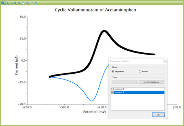
Figure 1. Selection of Only One CV Segment in AfterMath
Now you have extracted one segment of a CV to create a new one segment LSV plot (see Figure 2).
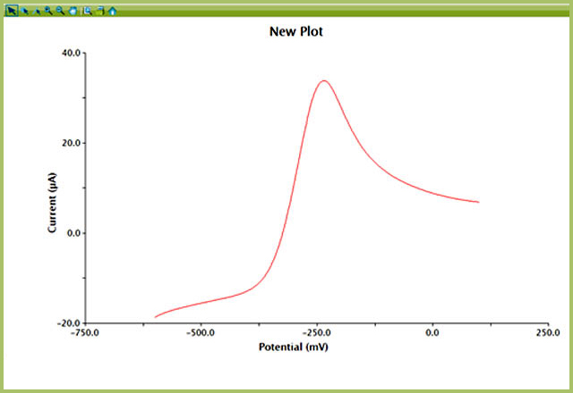
Figure 2. One Segment LSV Copied from Original CV Data
3.2Adjust Axes and Units as Desired
By default, AfterMath plots current (not current density) on the y-axis and potential on the x-axis. While this is fairly uniform across the electroanalytical community, the corrosion community typically reverses these axes. Prior to performing Tafel analysis, change any plotting orientations and units as desired.
3.2.1Adjusting Plot Axes
The corrosion community typically plots potential on the x-axis and current (or current density) on the y-axis. This is a simple “Basic Math Operations” Transform in AfterMath.
- Right click the LSV data on the plot and choose Apply Transform → Basic Math Operations… (see Figure 3)
- Select “Swap X/Y” Function. Ensure “Replace original trace” box is ticked under Options
- Press OK
Now potential will be on the x-axis and current will be on the y-axis.
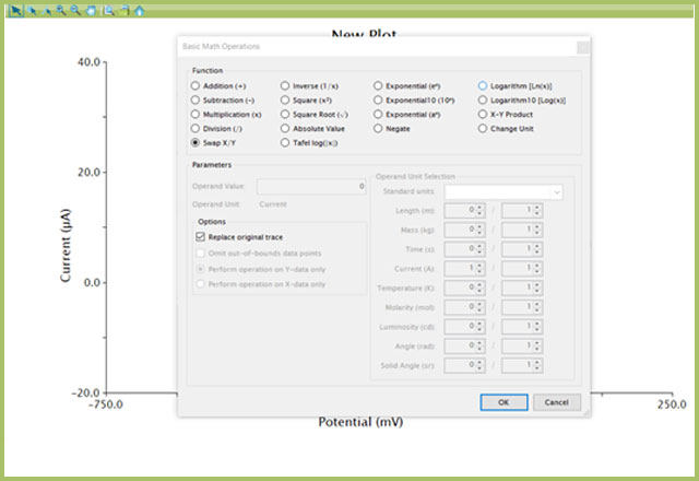
Figure 3. Use of Basic Math Operations to Transform Axes
3.2.2Plot x-axis as Current Density
Some scientists prefer to work in current density, which is simply the current divided by electrode area. By default, AfterMath does not perform this normalization and will always output current. With another simple “Basic Math Operations” Transform in AfterMath, current can be converted to current density.
- Right click the LSV data on the plot and choose Apply Transform → Basic Math Operations… (see Figure 4)
- Select “Division (/)” Function
- Enter Operand Value (i.e., the electrode area, in m2)
- Tick the “Replace original trace”
- Choose the appropriate radio button to perform this operation on the x-axis or y-axis
- Choose the axis displaying current
- Select "Area" from the Standard units drop-down in the Operand Unit Selection section
- Press OK
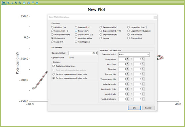
Figure 4. Use of Basic Math Operations to Convert Current to Current Density in AfterMath
Change the units on the current axis by double-clicking the axis to open the Axis Properties window. Here, untick “Automatic unit selection” under the Units section and choose the desired units to display (see Figure 5).
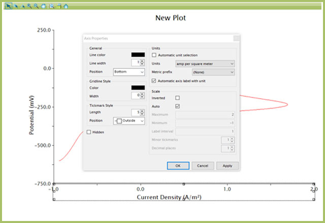
Figure 5. Adjustment of Unit Display on a Plot in AfterMath
3.3Convert to Tafel Plot (log current plot)
- Right-click the LSV data on the plot and choose Apply Transform → Basic Math Operations… (see Figure 6)
- Select “Tafel log (|x|)” Function
- Tick the “Replace original trace”
- Choose the appropriate radio button to perform this operation on the x-axis or y-axis. Choose the axis displaying current
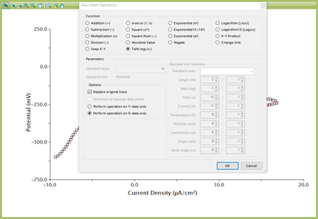
Figure 6. Use of Basic Math Operations to Transform Plot to Tafel Convention
The final result will be the correct form of a Tafel Plot (see Figure 7). In real-world systems, especially in the electrochemical corrosion field, the data may appear well-behaved, as shown in nearly all textbooks. Real-world systems may not always exhibit classic behavior. Realize the steps provided in this guide are simple arithmetic transformations and have not altered your data in any way. The transformations have only adjusted how the data are presented on a plot.
The next step is often to extract slope data for the anodic and cathodic components of the Tafel Plot, for use in corrosion rate calculations. Some users may simply use common estimates of these values, based on the corroding material. In other cases, researchers may wish to analytically determine the slope.
The next section will discuss how to extract the Tafel Slopes with simple tools.
4Slope Determination
AfterMath includes a variety of tools for data analysis. The “Baseline” option is useful for finding the slope about a series of data points. The Baseline tool can be used to extract the βa and βc values from the transformed Tafel Plot from Section 2.
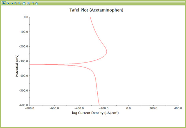
Figure 7. Tafel Plot Representation of Current vs Voltage Data
4.1Determine Tafel Slopes
Once the Tafel plot has been created (from CV or LSV data, as above), use the Baseline tool to find the slope about a section of data, selected by the user.
- Right click the LSV data on the plot and choose Add Tool → Baseline
- Adjust the two pink dots to the desired region of the curve where the slope should be calculated. The slope and intercept are calculated with each movement of the pink dots. Double-click the label for additional (but not required) options for formatting and display options of the tool results
- Repeat Steps 1 – 2 for the other slope on the Tafel Plot
The Tafel Plot with slope determination is now complete (see Figure 9). Adjust the view of the plot by double-clicking axes and manually setting the maximum, minimum, and label interval for optimal viewing.
Record the slope values for further use and calculations as needed. Saving the archive preserves all of the transformations and analyses performed and can be referenced at a later point.
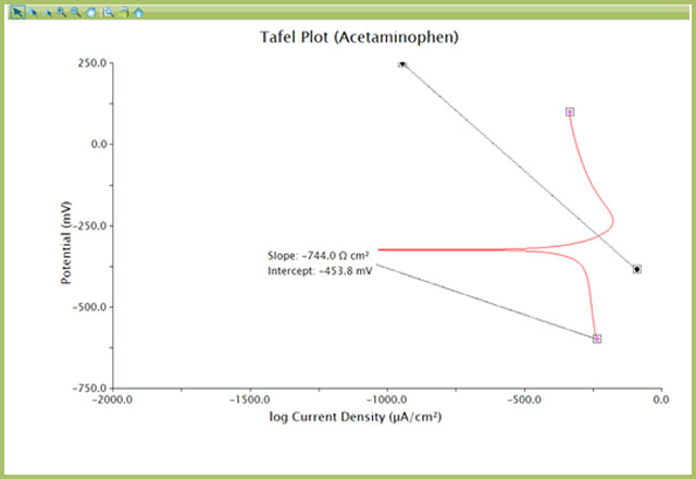
Figure 8. Addition of Baseline Tool to Tafel Plot for Slope Determination
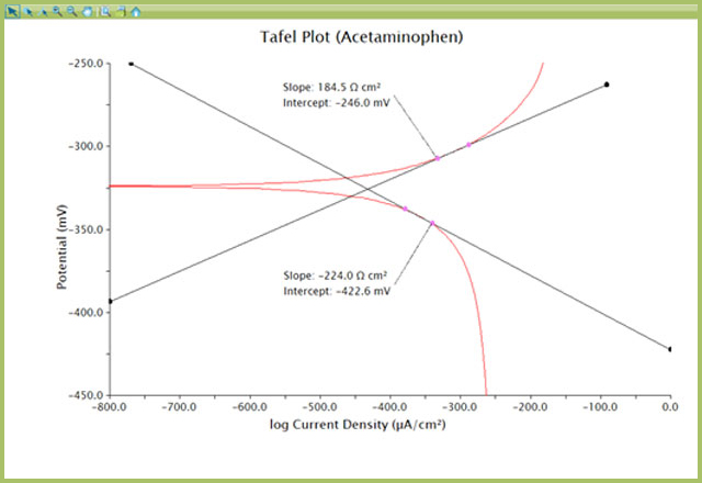
Figure 9. Tafel Plot with Slope Measurements (axes optimized for best data view)