This article is part of the AfterMath Data Organizer User’s Guide
-
AfterMath: Monitoring an Experiment in Progress
Read More -
AfterMath: Instrument Control
Read More
This article is part of the AfterMath Data Organizer User’s GuideThe AfterMath application periodically scans your computer system in search of any supported instruments. When an instrument is discovered, it is added to a list of available instruments. You can view the list of available instruments by clicking on the “Instruments” item as shown in the example below.
Most often, AfterMath is used to control only one instrument, so the Instrument List contains only one entry. But, in the example above, there are four different instruments being monitored (simultaneously) by the AfterMath software. Most of the instruments are idle, but one of them is in the middle of performing an experiment and actually has two additional experiments queued up for subsequent execution. Another one of the instruments is having a communications problem (perhaps the USB cable has been unplugged accidently). And finally, one of the instruments is a virtual instrument.The Instrument List is useful when you are using more than one instrument at the same time. The list gives you a snapshot summary regarding the status of all of the instruments.
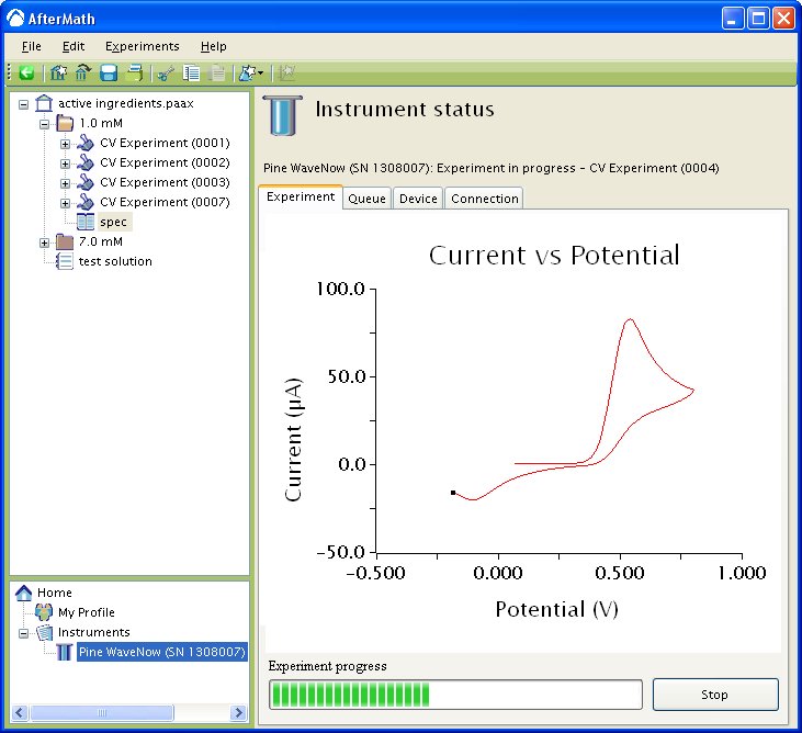
When you want more information about a specific instrument, you can double-click on the particular row of the Instrument List corresponding to that instrument. This brings up the detailed "Instrument Status" display for that particular instrument.
-
AfterMath: Data Tables
Read More
This article is part of the AfterMath Data Organizer User’s GuideSignals
A set of results from a single individual experiment is usually stored as a data table in an archive. Data tables contain two-dimensional relationships which record how various signal levels change during an experiment. A simple set of results might include time-dependent measurements of several signals, such as voltage vs. time, temperature vs. time, or current vs. time.
Somewhat more complex relationships between signals might also be recorded. For example, the data table might also include a record of how one signal (i.e., an excitation signal) influences another signal (i.e., a response signal). Examples of these kind of relationships include current vs. voltage or temperature vs. heating coil current.
Still more complex relationships might involve a bit of post-experiment computation (post-processing) using the raw data. For example, it may be useful to record the ratio of a voltage signal to a current signal vs. time (perhaps to indicate how an electrical resistance changed during the experiment). Or, it might be of interest to view how the current signal changes versus the square root of time (perhaps to elucidate how diffusion influences the measured current).
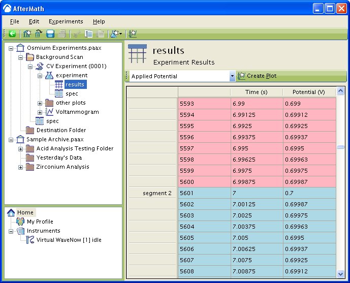
Regardless of the complexity of a signal relationship or how it is computed, this kind of two dimensional data is generally recorded as a set of ordered pairs, most often appearing as two columns of numeric data as shown in the figure below.
The data visible in the example (above) is a portion of a triangle waveform describing a voltage that was applied to an electrode during a voltammetry experiment. The voltage was recorded every 1.25 milliseconds, and the portion of data shown was measured about seven seconds into the experiment. Using the scroll bar along the side of the data table, it is possible to view data acquired at earlier or later points in the experiment.
Data Segments and Shading
The background shading in a data table often indicates additional information about a particular segment of the data. The default shading color is gray, but alternating pink and blue shading is often used to indicate the boundary between adjacent segments. In the example above, the pink shading indicates data recorded during the first segment of the triangle wave where the voltage signal is increasing versus time. The blue shading indicates the second segment of the triangle wave where the the voltage begins to decrease with time. In addition an entry is placed in the first column of the table to indicate the start of the second segment.
Orange shading is sometimes used to indicate data which is known to be invalid or flawed in some way.
Tables Containing Multiple Signals
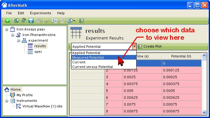
Many instruments produce more than one signal of interest during a given experiment. AfterMath groups all of the related signals from an experiment together into one data table in the archive. When you view a data table which contains more than one signal, it appears as shown below. There is a drop down list at the top of the display area which allows you to choose which signal relationship is displayed. In the example below, there are four different signal relationships which can be viewed.
Turning Signals into Plots
Scientists typically prefer to view signal measurements as traces on a plot rather than tables of numbers. If you would like to view a signal on a plot, simply click on the “Create Plot” button near the top of the table.
More details about this option are found later in this manual (click here).
Moving, Copying, Deleting, Importing
Moving and Copying Data Tables
In general, most AfterMath data tables are permanently bound to experiment results and cannot be individually moved or copied. AfterMath requires such data tables to remain linked together with the experiment specification that was used to generate the data (i.e., a data table by itself has no experimental context and is not allowed).
However, you can usually move or copy the entire experiment to which a data table belongs. When you copy the entire experiment, the data table and the experiment specification are both copied at the same time, so that the context of the data table is not lost.
Copying Data to Other Applications
You may copy data from a data table to another application by using the mouse to select some or all of the rows of the data table. Once these rows are selected, choose “Copy” from the file menu (or just press Control-C on the keyboard). This will copy the data from the selected rows to the system clipboard. You can then paste this numeric data into most major word processing and spreadsheet programs.
Deleting a Data Table
Because data tables are usually bound to a particular experiment, it is not possible to delete an individual data table. However, it is usually possible to delete the entire experiment from the archive. When you delete an experiment, both the data table and the experiment specification are removed from the archive.
Importing Data from Other Applications into a Data Table
Versions of the AfterMath software which are distributed for purposes of controlling and acquiring data from an instrument are generally not able to import data from other sources. Data tables are generated solely as the result of performing experiments and acquiring data from the instrument.
-
AfterMath: The Home View
Read More
This article is part of the AfterMath Data Organizer User’s GuideStarting with the Home View
Navigating Back to the Home View
Home View Options
The Home view offers 4 main actions: perform an experiment, open an archive, create a plot, and pine interactive. More information about each section is detailed below.
Perform an Experiment
This section of the Home view lists several very common experiments. To perform one of these experiments, simply click on the link for the desired experiment, and a new (blank) specification for that type of experiment is created in the archive. More about how to perform experiments on instruments can be found later in this manual (click here).
Open an Archive
This section of the Home view displays a list of links to the most recent archives that you have used. Clicking on one of these links automatically opens the archive so that you can view its contents.
There is also a link which allows you to create a new archive. If you click on this link, a new (unnamed and empty) archive is created. The new archive is not actually created on the hard drive unless you put some data into the archive and save it to a particular archive file.
Create a Plot
This section of the Home view lets you create a new plot (either an empty plot or a plot showing data from a previously opened archive).
Create an Empty Plot
This option simply creates a new (empty) plot in the archive. You can add traces to the plot by copying or dragging them from other plots.
Plot Existing Data
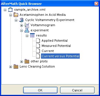
This option creates a new plot using data from a previously opened archive. When you click on this option, a dialog box appears (see below) which lets you select which data from the archive should be placed on the new plot.
Pine Interactive
This section of the Home view contains several useful links for navigating directly to Pine's web site. Use these links to send a message to Pine, to view Pine's commmercial e-commerce web site, or to reach the on-line AfterMath support site.
The main support page for the AfterMath Data Organizer software can be accessed directly from the Pine Interactive options.
The commercial web site for Pine Research Instrumentation can be accessed directly from the Pine Interactive options.
For additional assistance and convenience, researchers may wish to contact Pine Research Instrumentation directly.
AfterMath: Data Plots

This article is part of the AfterMath Data Organizer User’s Guide
Plots
 By far the most popular way scientists choose to view the results of an experiment is via a simple two-dimensional plot of the results. AfterMath has powerful plotting capabilities, allowing you to create simple or complex graphs from your experimental data.
A very simple plot residing in an archive is shown in the figure below. The plot has a title, axes, gridlines, and one single data trace on it. The plot could be made more complex by adding additional traces, adding one or more measurement tools, adding text boxes, or by adding additional axes (top axis and/or right axis) to the plot.
Moving and Copying Plots
As is the case with most other items in an archive, a plot may be moved, copied, or duplicated almost anywhere in the archive. You can also copy plots from one archive to another archive.
Copying Plots to Other Applications
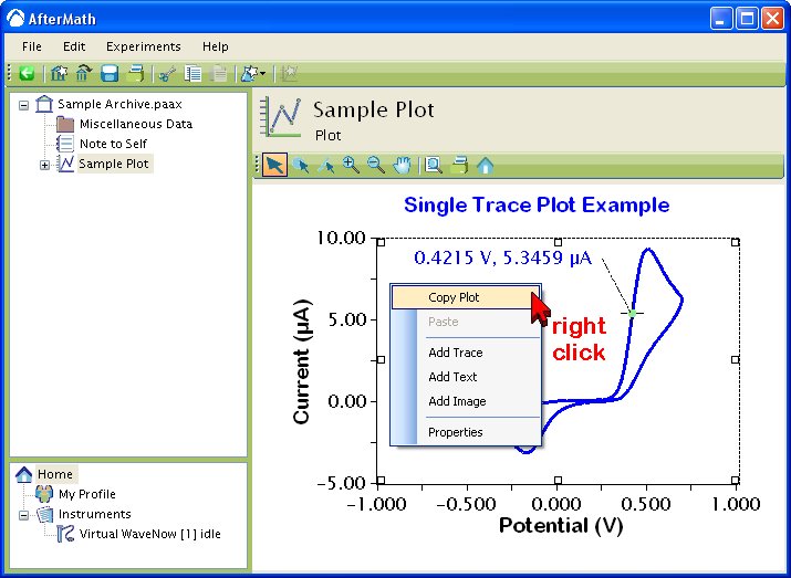
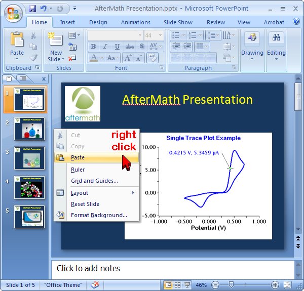
If you right-click on a plot and choose “Copy Plot” from the popup menu, then a bitmap image of the plot is placed on the system clipboard. This bitmap image may subsequently be pasted from the system clipboard into other applications, including many word processing documents, spreadsheets, and presentation files.
An example of copying a plot to a Microsoft Powerpoint presentation is detailed in two steps:
AfterMath: Experimental Results and Study Folders

This article is part of the AfterMath Data Organizer User’s Guide
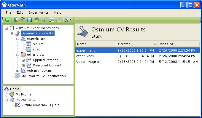
 When an experiment concludes, AfterMath places all of the results generated by the experiment into a special folder called a study folder. The study folder has a special icon which looks like a large paper clip. Inside a study folder you will find a read-only copy of the experiment results and specification along with one or more plots of the results. The precise contents of a study folder will vary depending upon the type of experiment you are performing.
The date and time that the experiment was performed can be deduced from the creation date of the items found in the study folder. Usually there is one main plot in the folder which is representative of the experimental results. In the example above, this main plot is called “Voltammogram”. Then, if there are any other plots related to the experiment, they are placed in the “Other Plots” folder.
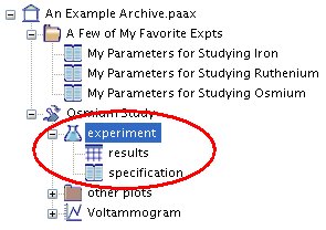 The raw data and the experiment specification are bound together underneath an icon which looks like a flask. The raw data is stored in a data table (named “results”) containing the measurements made during the experiment. The experiment specification (named “specification”) is a read-only copy of the parameters used to perform the experiment.
Unlike most other items found in an archive, AfterMath will not permit you to delete, move, or otherwise separate the experiment data from the experiment specification. The specification is “frozen” in a read-only state so that you do not accidently change the record of how the experiment was performed. However, AfterMath will permit you to make an “editable” copy of the experiment specification and store it somewhere else in the archive. Simply click on the “Create Copy” button at the top of the specification, and an “editable” copy will be created.
AfterMath: Experiment Specifications

This article is part of the AfterMath Data Organizer User’s Guide
Experimental Parameters
 When an experiment is performed on an instrument, two fundamental types of information become associated with that experiment. The most obvious information generated by the experiment is the raw data or set of measurements made by the instrument. The less obvious, but equally important, information associated with the experiment is how the experiment was performed (i.e., the set of parameters which specify how to do this experiment). These parameters, collectively called an experiment specification, must be configured ahead of time (by you) so that the AfterMath software (and the instrument being controlled by AfterMath) can perform the desired experiment.
 Once the experiment is completed, it is very important to bind together both the raw data and parameters which describe how the data was generated. This binding of experimental data with an experimental specification is strictly enforced by the AfterMath software.
When you look into an AfterMath archive which contains the results from a previously completed experiment, this strict binding is very apparent. In the example to the left, an experiment (represented graphically as a flask) contains two other items. The first item is a data table (named “results”) containing the measurements made during the experiment. The second item is an experiment specification (named “specification”) which is a record of the parameters used to make the measurements.
Unlike most other items found in an archive, AfterMath will not permit you to delete, move, or otherwise separate the experiment data from the experiment specification. The specification is “frozen” in a read-only state so that you do not accidently change the record of how the experiment was performed. However, AfterMath will permit you to make an “editable” copy of the experiment specification and store it somewhere else in the archive. The purpose of this editable specification is to give you an easy way to repeat the experiment using the same set of parameters, or if you wish, to make some modifications to the parameters in order to perform a slightly different, but related, experiment.
Editable vs. Frozen Specifications
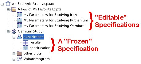
An reasonably sized archive is likely to contain many different experiment specifications. Some of these experiment specifications are likely to be bound to an experiment (“frozen”) while others are not bound to any experiment (“editable”). The latter might be humorously referred to as free range specifications as they are not confined to any one location in the archive and can be moved freely to any folder you wish.
In the example archive shown below, there are three freely “editable” specifications (located in the folder called “A Few of My Favorite Expts”), and there is one specification that is “frozen” because it is bound to the record of a previously completed experiment.
Editable specifications are usually the first kind of specification that you will create in an archive. When you are ready to configure a new experiment, you will first create a new “editable” specification which describes the experiment at some location in your archive. Then, you will issue a command to the instrument to perform the experiment. When the experiment is completed, AfterMath will automatically store the experiment results in the same location in the archive. AfterMath automatically makes a “frozen” copy of the specification and binds it to the experiment results.
Editable specifications are quite useful in those situations where you perform experiments with the same parameters over and over again. You can use an editable specification to store these parameters, and then reuse the same specification repeatedly to perform a series of identical experiments.
Creating an Editable Specification
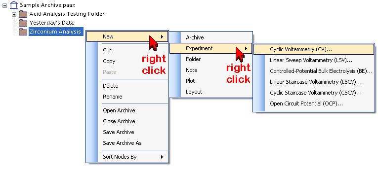
An editable experiment specification can be created in an archive by right-clicking on the folder in which you would like to place the specification. Choose the “New»Experiment” option from the popup menu (see below), and then select the kind of experiment you wish to configure. In the example below, a new specification for a cyclic voltammetry experiment is created.
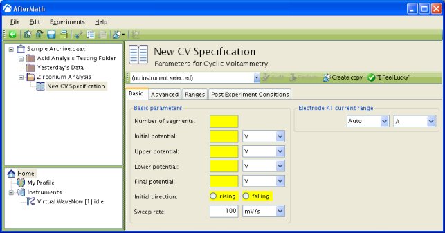
Once the new specification has been created, you may edit the parameters in the main viewing area. Parameters which are shaded in yellow are mandatory. If you provide an invalid value for a parameter, it will be shaded in pink. If you would like a set of default parameters to be provided by the software, click on the “I Feel Lucky” button.
The “Basic” tab on an experiment specification contains those parameters which are most often needed. The other tabs generally hold more advanced options which are not as frequently changed.
AfterMath: Data Folders

This article is part of the AfterMath Data Organizer User’s Guide
Folders
Within the tree-like structure of an archive, you are free to create folders in which to organize your data. Each folder is represented by the symbol shown to the left. You may also create folders within folders so that your archive has a multi-level internal structure.
Creating a Folder
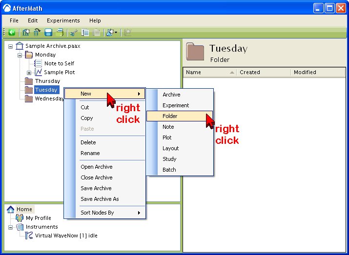
A folder is created with a right-click on an existing folder or archive in the “tree control” on the left side of the screen (see figure below). When you right-click on a folder or archive, a popup menu appears. Select the “New Folder” option from the popup menu.
A new folder is always created on the level just below the folder or archive on which you right-clicked. Once you have created a folder, you may move it to any location you wish.
Moving and Copying Folders
As is the case with most other items in an archive, a folder may be moved, copied, or duplicated almost anywhere in the archive using standard cut, copy, and paste methods or using drag-n-drop mouse actions.
You can also copy folders from one archive to another archive. When you move or copy a folder, the folder plus its entire contents are moved or copied.
Deleting a Folder
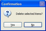
You may delete a folder by simply selecting it in the “tree control” and pressing the “Delete” key on your computer's keyboard. You will receive one warning message before the folder is deleted (see below).
Once you have deleted a folder and saved the archive, there is no way to recover the information. Be very sure that you want to delete a folder before you delete it.
There is one case where you may be able to recover from an accidental deletion of a folder. This case only applies if you are working with a previously saved archive which happened to contain the folder already. If you accidently delete such a folder and immediately realize the mistake, then DO NOT SAVE THE ARCHIVE to your hard drive. Instead, choose the “Save As” command from the “File” menu and save the archive using a different name. Then, reopen the archive with the original filename, and the folder should still be there.
AfterMath: Report Layouts

This article is part of the AfterMath Data Organizer User’s Guide
Using Report Layout
Most of the individual items in an archive have a printable representation suitable for sending to a hard copy printer. When you print an individual item in this manner, you are only able to print one item per page. Sometimes, it is desirable to print more than one item per page. For example, you may wish to put a plot of some experimental results at the top of a page and also include a list of the experimental parameters at the bottom of the same page.
When you want to print more than one item per page, you need to create a page layout. Proper page layout preoccupies the mind of many a graphics designer, but most scientists have fairly simple needs when it comes to reporting results in hard copy form. AfterMath lets you configure a grid-based layout using one of several standard international page sizes.
Creating a new Layout
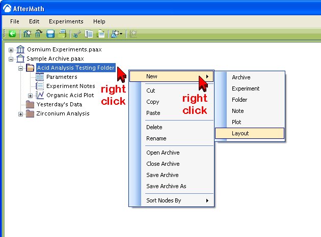
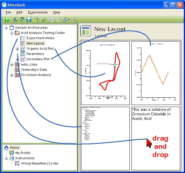
Creating an AfterMath layout involves choosing a paper size, deciding how many grid elements are needed on the page, and then literally dragging the items from the archive on to the various grid elements. This last step is performed using drag-n-drop mouse actions.
Step 1
The first step in creating a new layout is to decide where in the archive to put the layout. In general, it is good practice to copy all of the items that will appear on a layout into the same folder and then create a new layout item in that very same folder. In the example below, several items have been copied into a folder called “Acid Analysis Testing Folder”. A new layout is created in the folder by right-clicking on the folder and choosing “New » Layout” from the popup menu.
Step 2
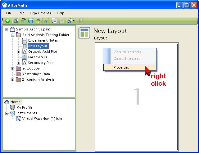
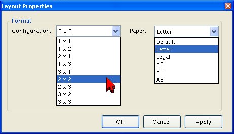
By default, a new (empty) layout has only one grid element which consumes the entire page. You can change the number of grid elements (and the paper size) by right-clicking on the layout and choosing the “Properties” option.
On the “Layout Properties” box, there are a variety of grid configurations available, allowing you to place anywhere from one to nine different items on the page.
Moving and Copying
Once you have created a layout, you can move it to any location within the same archive that you wish. But it is usually a good idea to keep it in the same folder as the items which you have placed on the layout (see note below).
AfterMath: Notes

This article is part of the AfterMath Data Organizer User’s Guide
Archive Notes
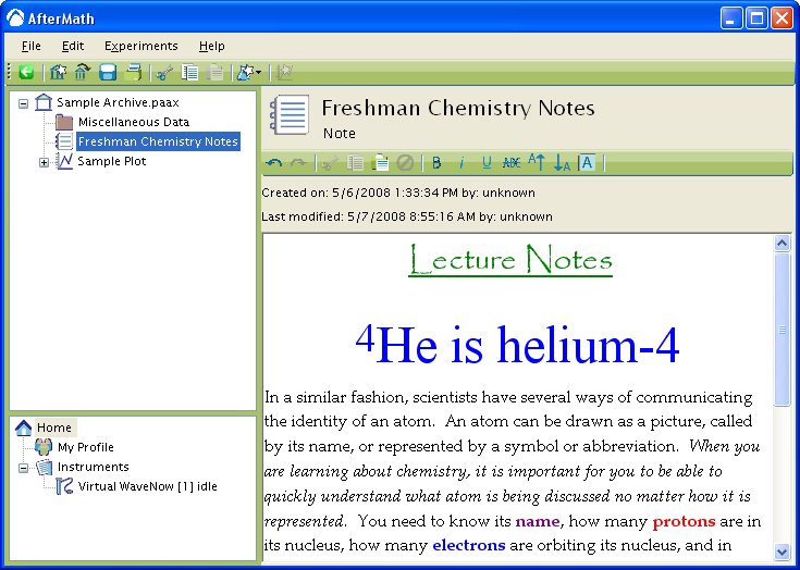
All scientists need to write down notes as they are performing laboratory experiments. While most of these notes should eventually find their way into a traditional laboratory notebook, it is often helpful to add notes to computer-based data files as you are acquiring data from an instrument. AfterMath allows you to add one or more notes, like the one shown in the figure below, to any item in an archive. AfterMath notes support multiple fonts, styles, and colors and many text formatting options which are important to scientists, such as superscripts and subscripts.
Note Creation
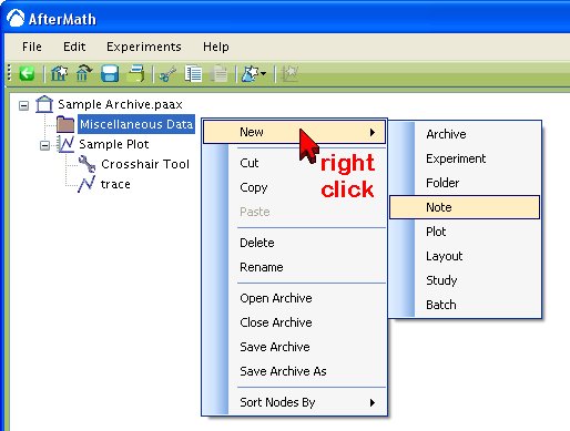
A note may be attached to any item in the archive. Simply right-click on any existing item in the archive in the “tree control” on the left side of the screen (see figure below). When you right-click on the item, a popup menu appears. Select the “New » Note” option from the popup menu.
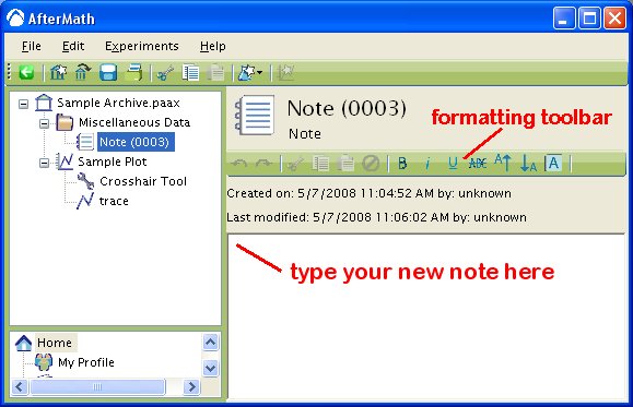
The action described above will attach a new note to the item you selected. Once the new note is created, you may edit it in the Main Viewing Area on the right side of the screen (see figure below).
Cut, Copy, Paste, Delete
Moving and Copying Notes
As is the case with most other items in an archive, a note may be moved, copied, or duplicated almost anywhere in the archive using standard cut, copy, and paste methods or using drag-n-drop mouse actions. You can also copy notes from one archive to another archive.
You may copy all or a portion of a note to the system clipboard and then paste that text into other applications.
Note Deletion
You may delete a note by simply selecting it in the “tree control” and pressing the “Delete” key on your computer's keyboard. You will receive one warning message before the note is deleted.
Pasting Text from Other Applications into a Note
You may copy text from another application to the system clipboard and then paste that text into a note. Some formatting in the original text may be lost, especially if you are copying text from a web browser. Also, any images embedded in the text will be removed.


