Uncategorized – Page 21 – Pine Research Instrumentation Store

Square Wave Voltammetry (SWV)

This article is part of the AfterMath Data Organizer Electrochemistry Guide

The difference current between a forward and reverse pulse is plotted as a function of potential to yield a voltammogram.

Detailed Description

Like most of the other electrochemical techniques offered by the AfterMath software, Square Wave Voltammetry (SWV) begins with an induction period. During the induction period, a set of initial conditions is applied to the electrochemical cell and the cell is allowed to equilibrate to these conditions. The default initial condition involves holding the working electrode potential at the Initial Potential for a brief period of time (i.e., 3 seconds).

After the induction period, the potential of the working electrode is stepped through a series of forward and reverse pulses from the Initial potential to the Final potential. The forward step is determined by the Square amplitude and the reverse step is determined by subtracting the Square increment from the Square amplitude. Cyclic Square Wave Voltammetry (CSWV) is a variant where the potential of the working electrode is cycled between an Upper potential and a Lower potential.

After the pulse sequence has finished, the experiment concludes with a relaxation period. The default condition during the relaxation period involves holding the working electrode potential at the final potential for an additional brief period of time (i.e., 1 seconds).

At the end of the relaxation period, the post experiment idle conditions are applied to the cell and the instrument returns to the idle state.

Difference current between the forward and reverse pulses is plotted as a function of the potential applied to the working electrode, resulting in a voltammogram.

Parameter Setup

The parameters for this method are arranged on various tabs on the setup panel. The most commonly used parameters are on the Basic tab, and less commonly used parameters are on the Advanced tab. Additional tabs for Ranges and Post experiment idle conditions are common to all of the electrochemical techniques supported by the AfterMath software.

Basic Tab

For SWV, you can click on the “I Feel Lucky” button (located at the top of the setup) to fill in all the parameters with typical default values (see Figure 1). You may need to change the Initial potential and Final potential, to values which are appropriate for the electrochemical system being studied.

Figure 1 : Basic setup for SWV.

The waveform that is applied to the electrode is a series of forward and reverse pulses (see Figure 2) each having an amplitude of Square amplitude and incremented according to the Square increment. The total time for the forward and reverse pulses is the Square period. Using the sample waveform below, the first pulse is $25 \; mV$ in the positive direction for $5 ms$ . The current is sampled (red squares) during the forward pulse at the time obtained by subtracting the Sample width from $1/2$ of the Square period. The potential of the working electrode is then stepped to $-25 \; mV$ for $5 \; ms$ . The current is then measured (black squares) at the time obtained by subtracting the Sample width from the Square period.

Figure 2: Zoom of waveform for SWV.

Advanced Tab

The Advanced Tab for this method allows you to change the behavior of the potentiostat during the induction period and relaxation period. By default, the potential applied to the working electrode during the induction and relaxation period will match the initial potential and final potential, respectively, as specified on the Basic Tab. You may override this default behavior, and you may also change the durations of the induction and relaxation periods if you wish.

Ranges Tab

Though AfterMath has the ability to automatically select the appropriate ranges for voltage and current during an experiment it is best to manually select the current range for any pulse technique. Please see the separate discussions on autoranging and the Ranges Tab for more information.

Post Experiment Conditions Tab

After the Relaxation Period, the Post Experiment Conditions are applied to the cell. Typically, the cell is disconnected but you may also specify the conditions applied to the cell. Please see the separate discussion on post experiment conditions for more information.

Typical Results

Typical results for a $1 \; mM$ solution of Ferrocene in $0.1 \; M \; Bu_4NClO_4/CH_2Cl_2$ are shown below (see Figure 3, specific SWV parameters were: $25 \; mV$ square amplitude, $2 \; mV$ square increment, $10 \; ms$ square period, $1 \; ms$ sample width). Also included are plots of the forward (see Figure 4A) and reverse (see Figure 4B) currents. Notice that the each looks like a typical LSV curve, with the forward being an oxidation and the reverse being the reduction. Please see the Theory section for more information.

Figure 3:Square Wave Voltammogram of a Ferrocene Solution

Figure 4: A) Forward current and B) Reverse current of a Ferrocene Solution

Below is an example for CSWV of a $1 \; mM$ solution of Ferrocene in $0.1 \; M \; Bu_4NClO_4/CH_2Cl_2$ (see Figure 5, specific parameters were: $25 \; mV$ square amplitude, $2 \; mV$ square increment, $10 \; ms$ square period, $1 \; ms$ sample width). Peak potentials are marked with a Crosshair tool to show that the anodic and cathodic peaks appear at nearly the same potential.

Figure 5 : Cyclic Square Wave Voltammogram for a Ferrocene Solution

Theory

The following is a brief introduction to the theory of SWV. SWV was invented by Ramaley and Krause¹. Please see Bard and Faulkner², Osteryoung and O'Dea ³ or Osteryoung and Osteryoung⁴ for additional information on the technique. CSWV, originally developed by Xinsheng and Guogang⁵, and recently revived by Helfrick and Bottomley⁶, is covered in the literature also.

SWV combines the aspects of several pulse voltammetric methods, including the background supression and sensitivity of DPV, the diagnostic value of NPV, and the ability to interrogate products directly in the manner of RNPV.

Consider a reaction $O + e^- \rightarrow R$ , where $O$ is reduced in a one electron reaction to $R$ with formal potential, $E^{0}$ . An initial potential is applied to the electrode that is significantly more positive than $E^{0}$ . No significant faradaic current flows upon the application of forward pulse towards more negative values. Current is sampled at a specified point during the forward pulse.

The reverse pulse consists of stepping the potential of the working electrode to more positive values and the current is sampled near the end of the reverse pulse. The difference current is calculated by subtracting the reverse current from the forward current.

As the potential of the working electrode approaches $E^{0}$ a faradaic current flows due to reduction of $O$ . Upon application of the reverse pulse, a faradaic current flows in that effectively oxidizes the $R$ was was produced during the forward pulse. In other words, the rate of reduction slows compared to the forward step, hence an anodic current flows. Once the potential of the working electrode is sufficiently more negative of $E^{0}$ the current is diffusion-limited in both the forward forward and reverse pulses and the difference current is small.

SWV's strengths lie in diagnostics, meaning that it is not typically used for quantitation. It is possible however, to calculate peak height using the equation

${\Delta}i_p = \frac{nFAD_O^{1/2}C_O^*}{{\pi}^{1/2}t_p^{1/2}}{\Delta}{\psi}_p$

where $n$ is the number of electrons, $F$ is Faraday's Constant ( $96485 \; C/mol$ ), $A$ is the electrode area ( $cm^2$ ), $D_{0}$ is the diffusion coefficient of species $O$ ( $cm^2/s$ ), $C_O$ is the concentration of species $O$ ( $mol/cm^3$ ), $t_p$ is the experimental time scale ( $1/2$ Square period – Sample window), and ${\Delta}{\psi}_p$ is a Dimensionless Peak Current parameter (see Table 1).

Table 1. Dimensionless Peak Current ( ${\Delta}{\psi}_p$ ) vs. SWV Operating Parameters^a

$n{\Delta}E_i/mV$

$n{\Delta}E_a/mV$ $1$ $5$ $10$ $20$

$0^b$ $0.0053$ $0.0238$ $0.0437$ $0.0774$

$10$ $0.2376$ $0.2549$ $0.2726$ $0.2998$

$20$ $0.4531$ $0.4686$ $0.4845$ $0.5077$

$50$ $0.9098$ $0.9186$ $0.9281$ $0.9432$

$100$ $1.1619$ $1.1643$ $1.1675$ $1.1745$

^aData from reference 3.
${\Delta}E_a$ = Square amplitude
$^b{\Delta}E_a = 0$ corresponds to SCV
${\Delta}E_i$ = Square increment

Applications

The first application uses SWV to monitor binding events associated with electrochemical sensors. White and Plaxco⁷ developed redox-tagged electrochemical sensors from electrode-bound oligonucleotides. Tuning the frequency of the voltammetric measurements allows the researchers to amplify both the unbound and target-bound signals, essentially, making an “On/Off” sensor.

The second example used several electrochemical techniques, SWV among them, to monitor metal dissociation events. Chakrabarti et al.⁸ combined RDE with anodic stripping voltammetry to distinguish between labile and nonlabile complexes in extremely low concentrations in aqueous solutions and in precipitation samples. The authors then showed that DPV, SCV and SWV all give similar dissociation constants but SWV's sensitivity was two orders of magnitude higher than SCV. This is a nice example of how SWV compares with other electrochemical techniques.

References

1. Ramaley, L.; Krause, Jr., M. S. Anal. Chem. 1969, 41, 1365–1369.

2. Faulkner, L. R.; Bard, A. J. Polarography and Pulse Voltammetry, Electrochemical Methods: Fundamentals and Applications, 2^nd ed.; Wiley: New Jersey, 2000; 261-304.

3. Osteryoung, J.; O'Dea, J. J. Electroanal. Chem. 1986, 14, 209.

4. Osteryoung, J.; Osteryoung, R. A. Anal. Chem. 1985, 57, 101A–110A.

5. Xinsheng, C.; Guogang, P. Anal. Lett. 1987, 20, 1511-1519.

6. Helfrick, Jr., J. C.; Bottomley, L. A. Anal. Chem. 2009, 81, 9041-9047.

7. White, R. J.; Plaxco, K. W. Anal. Chem. 2010, 82, 73-76.

8. Chakrabarti, C. L.; Cheng, J.; Lee, W. F.; Back, M. H.; Schroeder, W. H. Environ. Sci. Technol. 1996, 30, 1245–1252.

Additional Resources

Links: Electrochemist's Guide, AfterMath User's Guide, AfterMath Main Support Page

Related Techniques: Differential Pulse Voltammetry (DPV), Normal Pulse Voltammetry (NPV), Reverse Normal Pulse Voltammetry (RNPV)

Posted 1/4/2016 in Uncategorized
Read More
Post-Experiment Idle Conditions

This article complements the AfterMath Data Organizer Electrochemistry Guide

When an experiment concludes, the instrument reverts to its idle mode and applies a set of idle conditions to the electrochemical cell.

By default, the instrument simply disconnects from the electrochemical cell.

You may override this default behavior by specifying an alternate set of conditions on the Post-Experiment tab on the form shown below. In the example below, the first working electrode is placed under galvanostatic control after the experiment concludes, and a signal level ( $\text{-470 mA}$ ) is applied to the electrode. The second working electrode is placed under potentiostatic control, and a signal level ( $\text{+340 mV}$ ) is applied to the electrode.

Links: Electrochemist's Guide, AfterMath User's Guide, AfterMath Main Support Page

Related Topics: cell switching, relaxation period, idle conditions

Posted 1/4/2016 in Uncategorized
Read More
Range Tab

This article is part of the AfterMath Data Organizer Electrochemistry Guide

Autoranging

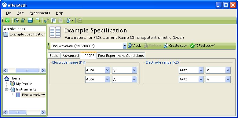
The choice of measurement sensitivity for the potential and current signals is made on the Ranges Tab. By default, both these range settings are set to “Auto”, meaning that the software and/or instrument will attempt to choose an appropriate signal sensitivity automatically. This is referred to as the “autorange” feature.

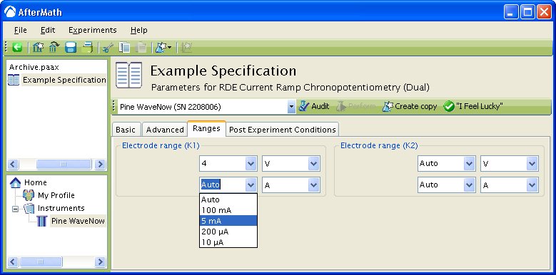
Figure 1: Choosing Specific Ranges

In the example shown above (see Figure 1), the potential and current ranges on the second working electrode are set to autorange.

The potential range on the first working electrode has been manually set to $\text{4.0 volts}$ , meaning that the user expects the working electrode potential to stay within the range from $\text{-4.0 volts}$ to $\text{+4.0 volts}$ throughout the entire experiment.

Also in the example above, the user is in the process of selecting a current range for the first working electrode from a drop-down menu. The four choices shown in the menu ( $\text{100 mA, 5 mA, 200} \; {\mu}A,$ and $10 \; {\mu}A$ ) are the four available ranges on the Pine WaveNow potentiostat. If a different potentiostat system were in use, then the choices in this drop-down menu would likely be different.

Overriding Autorange

In some cases, you will need to override the “Auto” range feature and select a particular range that is known to be appropriate for the particular electrochemical system you are studying. Consider a $\text{1 mM}$ solution of $K_3Fe(CN)_6$ in $\text{0.1 M KCl}$ ( $\text{3 mm}$ disc GC working electrode and sweep rate $\text{100 mV/s}$ ). If the choice of electrode range is too small (i.e. $10 \; {\mu}A$ ), actual current may go off scale and be truncated (see Figure 2, red trace). If the electrode range is too large (i.e. $\text{5 mA}$ ), the voltammogram may have a noisy, choppy, or quantized appearance (see Figure 2, black trace). If the correct electrode range is chosen (i.e. $200 \; {\mu}A$ ), the voltammogram is smooth (see Figure 2, green trace).

Figure 2: Influence of Current Range Choice on Voltammogram Quality

Not all instruments support the “autorange” feature. For instruments which do not support this feature, choosing the “Auto” range setting usually causes the least sensitive range setting to be selected.

Additional Resources

Links: Electrochemist's Guide, AfterMath User's Guide, AfterMath Main Support Page

Related Topics: autoranging

Posted 1/4/2016 in Uncategorized
Read More
Ranges

This article complements the AfterMath Data Organizer Electrochemistry Guide

The “Ranges” tab is set to Autorange by default (see below).

To change the default settings, simply choose the wanted potential or current range from the drop down menu. In the example below, $\text{4 volts}$ has already been selected and the user is in the process of changing the Auto current range to $\text{5 mA}$ .

Links: Electrochemist's Guide, AfterMath User's Guide, AfterMath Main Support Page

Posted 1/4/2016 in Uncategorized
Read More
Normal Pulse Voltammetry (NPV)

This article is part of the AfterMath Data Organizer Electrochemistry Guide

Detailed Description

Like most of the other electrochemical techniques offered by the AfterMath software, this experiment begins with an induction period. During the induction period, a set of initial conditions is applied to the electrochemical cell and the cell is allowed to equilibrate to these conditions. The default initial condition involves holding the working electrode potential at the Baseline Potential for a brief period of time (i.e., 3 seconds).

After the induction period, the potential of the working electrode is stepped through a series of pulses from the Initial potential to the Final potential. The potential is incremented with each successive pulse according to the Pulse increment. Current is measured at the time obtained by subtracting the Sample window from the Pulse width. Cyclic Normal Pulse Voltammetry (CNPV) consists of a cycling (through a series of potential pulses also) the potential of the working electrode between an Upper potential and a Lower potential. Reverse Normal Pulse Voltammetry (RNPV) is a variant of NPV where you choose to apply a Baseline potential in a region where faradaic current is flowing at a maximal rate ( $>200 \; mV$ from $E^0$ ).

After the pulse sequence has finished, the experiment concludes with a relaxation period. The default condition during the relaxation period involves holding the working electrode potential at the Final potential for an additional brief period of time (i.e., 1 seconds).

At the end of the relaxation period, the post experiment idle conditions are applied to the cell and the instrument returns to the idle state.

Current is sampled during each pulse and is plotted as a function of the potential applied to the working electrode, resulting in a voltammogram.

Parameter Setup

The parameters for this method are arranged on various tabs on the setup panel. The most commonly used parameters are on the Basic tab, and less commonly used parameters are on the Advanced tab. Additional tabs for Ranges and Post experiment idle conditions are common to all of the electrochemical techniques supported by the AfterMath software.

Basic Tab

For NPV, you can click on the “I Feel Lucky” button (located at the top of the setup) to fill in all the parameters with typical default values (see Figure 1). You may need to change the Baseline potential, Initial potential and Final potential, to values which are appropriate for the electrochemical system being studied.

Figure 1: Basic setup for NPV.

There is no separate Experiment to choose for RNPV, rather you are entering the parameters so as to begin in a region where a faradaic current flows at a maximal rate ( $>200 \; mV$ from $E^0$ ) upon application of the Baseline potential. You can click on the “I Feel Lucky” button (located at the top of the setup) to fill in all the parameters with typical default values (see Figure 2). You will likely need to change the Baseline potential, Initial potential and Final potential, to values which are appropriate for the electrochemical system being studied.

Figure 2: Basic setup for RNPV.

For CNPV, you can click on the “I Feel Lucky” button (located at the top of the setup) to fill in all the parameters with typical default values (see Figure 3). You may need to change the Baseline potential, Number of segments, Initial potential, Upper potential, Lower potential, and Final potential, to values which are appropriate for the electrochemical system being studied.

If you choose any odd number of segments greater than two, the parameters that must be entered are a little different than the two segment case. You must choose a Baseline potential, Initial Potential, Upper Potential, Lower Potential, and Final potential. You must also choose whether the Initial direction is rising (pulses toward Upper Potential) or falling (pulses toward Lower Potential). If the Initial direction is rising, the Final potential must be different than the Lower potential. If the Initial direction is falling, the Initial potential must be different than the Lower potential.

If you choose any even number of segments greater than two, the parameters that must be entered are the same as the three segment case. You must choose an Baseline potential, Initial Potential, Upper Potential, Lower Potential, and Final potential. You must also choose whether the Initial direction is rising (pulses toward Upper Potential) or falling (pulses toward Lower Potential). If the Initial direction is rising, the Final potential must be different than the Upper potential. If the Initial direction is falling, the Initial potential must be different than the Lower potential.

Figure 3: Basic setup for CNPV.

The waveform that is applied to the electrode for all three techniques consists of a series of Pulse periods with a potential step, for a specified time, from a baseline potential near the end of each period (see Figure 4). The potential step is incremented with each period until the final potential is reached. During each potential pulse, the current is measured at a specified time before the end of the pulse. For CNPV, the pulse sequence starts at the Initial potential and is then cycled between the Upper potential and Lower potential for one less than the specified number of segments. The final segment steps from the Upper potential or Lower potential to the Final potential depending if the Initial direction was rising or falling.

Figure 4 : Waveform. Orange trace – applied potential, red squares – current sampled. A: Waveform. B: Zoom of Waveform.

Advanced Tab

The Advanced Tab for this method allows you to change the behavior of the potentiostat during the induction period and relaxation period. By default, the potential applied to the working electrode during the induction and relaxation period will match the initial potential and final potential, respectively, as specified on the Basic Tab. You may override this default behavior, and you may also change the durations of the induction and relaxation periods if you wish.

Ranges Tab

Though AfterMath has the ability to automatically select the appropriate ranges for voltage and current during an experiment it is best to manually select the current range for any pulse technique. Please see the separate discussions on autoranging and the Ranges Tab for more information.

Post Experiment Conditions Tab

After the Relaxation Period, the Post Experiment Conditions are applied to the cell. Typically, the cell is disconnected but you may also specify the conditions applied to the cell. Please see the separate discussion on post experiment conditions for more information.

Typical Results

The typical results for NPV of a $0.5 \; mM$ solution of Ferrocene in $0.1 \; M \; Bu_4NClO_4/MeCN$ show a sigmoid-shaped curve (see Figure 5, specific parameters were: $2 \; mm$ Pt WE, Pt mesh CE, Baseline Potential = $0.1 \; V$ , Initial Potential = $0.25 \; V$ , Final Potential = $1 \; V$ , Pulse increment = $10 \; mV$ , Pulse period = $100 \; ms$ ,Pulse width = $10 \; ms$ , Sample width = $1 \; ms$ ).

Figure 5: Typical NPV results for $0.5 \; mM$ Ferrocene in $0.1 \; M \; Bu_4NClO_4/MeCN$

The typical results for RNPV of the same $0.5 \; mM$ Ferrocene in $0.1 \; M \; Bu_4NClO_4/MeCN$ also show a sigmoid-shaped curve (see Figure 6, specific parameters were: Baseline Potential = $1 \; V$ , Initial Potential = $0.75 \; V$ , Final Potential = $0 \; V$ , Pulse increment = $10 \; mV$ , Pulse period = $100 \; ms$ ,Pulse width = $10 \; ms$ , Sample width = $1 \; ms$ ).

Figure 6: Typical RNPV results for a Ferrocene Solution.

Finally, the typical results for CNPV (two segments) of the same $0.5 \; mM$ Ferrocene in $0.1 \; M \; Bu_4NClO_4/MeCN$ show two sigmoid-shaped curves (see Figure 7, same conditions as Figure 6). Since Ferrocene is fully-reversible electrochemically, the two sigmoids overlap.

Figure 7: Typical CNPV results for a Ferrocene Solution.

Theory

The following is a brief introduction to the theory of NPV. Please see Bard and Faulkner¹ for additional information on the technique. NPV is a derivative technique of Normal Pulse Polarography (NPP). NPP is a technique that was traditionally used with Dropping Mercury Electrodes and Static Mercury Dropping Electrodes. The waveform for the two techniques is the same, however it is appropriate to use the term “Normal Pulse Voltammetry” when referring to the application of the waveform to nonpolarographic electrodes.

Consider a reaction $O + e^- \rightarrow R$ , where $O$ is reduced in a one electron reaction to $R$ with formal potential $E^0$ >. The application of a baseline potential should be sufficiently positive of $E^0$ such that no faradaic current flows. After a period of time ( $100$ – $5000 \; ms$ ), ${\tau}'$ , the potential of the working electrode is stepped to a more negative value for some time. The total time from the application of the baseline potential through the application of the potential pulse is ${\tau}$ .

The potential pulse is incrementally increased with each cycle. As the potential of the working electrode approaches $E^0$ faradaic current flows due to the reduction of $O$ to $R$ . Upon the application of the baseline potential in the next cycle, $R$ is oxidized back to $O$ . When the potential of the working electrode gets sufficiently negative of $E^0$ , $O$ is reduced to $R$ at a maximum rate and the current plateaus. The magnitude of this current plateau is given by

$i_{d,NPV} = \frac{nFAD_O^{1/2}C_O^*}{{\pi}^{1/2}({\tau}-{\tau}')^{1/2}}$

where $n$ is the number of electrons, $F$ is Faraday's Constant ( $96485 \; C/mol$ ), $A$ is the electrode area ( $cm^2$ ), $D$ is the diffusion coefficient( $cm^2/s$ ), $C$ is the concentration ( $mol/cm^3$ ) and ${\tau}'$ and ${\tau}$ are as described above.

As seen in the Typical Results section, RNPV gives the same wave shape but not the same current. These results are analogous to DPSCA where the current during the forward pulse is different than the current in the reverse pulse. Here in RNPV, the baseline potential is such that $O$ is being reduced to $R$ at a maximum rate. As the potential of the working electrode approaches $E^0$ a faradaic current flows due to the oxidation of $R$ to $O$ . Once the potential of the working electrode is sufficiently positive of $E^0$ , $R$ is being oxidized at a maximum rate and the current plateaus. The magnitude of this current plateau is give by

$i_{d,RPV} = \frac{nFAD_O^{1/2}C_O^*}{{\pi}^{1/2}}\left[{\frac{1}{({\tau}-{\tau}')^{1/2}}}-{\frac{1}{{\tau}^{1/2}}}\right]$

where the parameters are as described above. Notice that in the Typical Results section, there is a slight anodic current flowing at the beginning of the experiment. The magnitude of this current is given by the equation

$i_{d,DC} = \frac{nFAD_O^{1/2}C_O^*}{{\pi}^{1/2}{\tau}^{1/2}}$

where the parameters are as described above. The magnitude of this current is the difference between the NPV and RNPV currents.

Application

The first example uses NPV to confirm a diffusion coefficient calculated initially by CA. Oyaizu et al.² produced an organic radical polymer to be used in charge-storage applications. The current in this case is controlled by diffusion of the counter ion through the film.

The second example also uses NPV to measure a diffusion coefficient. Welch et al.³ measured the diffusion coefficients of a free and DNA-bound organo-metallic complex. NPV was superior to CV in this instance due to the low concentration of species in solution.

The next example uses RNPV. RNPV's useless lies in its ability to examine products from chemical reactions that take place after an electrochemical reaction. Osteryoung et al.⁴ used RNPV to obtain the backwards rate constant and equilibrium constant for the dimerization of N-methyl-2-carbomethoxypyridinium radical, produced after the electrochemical reduction of the N-methyl-2-carbomethoxypyridinium ion.

References

1. Faulkner, L. R.; Bard, A. J. Polarography and Pulse Voltammetry, Electrochemical Methods: Fundamentals and Applications, 2^nd ed.; Wiley: New Jersey, 2000; 261-304.

2. Oyaizu, K.; Ando, Y.; Konishi, H.; Nishide, H. J. Am. Chem. Soc. 2008, 130, 14459–14461.

3. Welch, T. W.; Corbett, A. H.; Thorp, H. H. J. Phys. Chem. 1995, 99, 11757–11763.

4. Osteryoung, J.; Talmor, D.; Hermolin, J.; Kirowa-Eisner, E. J. Phys. Chem. 1981, 85, 285–289.

Additional Resources

Links: Electrochemist's Guide, AfterMath User's Guide, AfterMath Main Support Page

Related Techniques: Differential Pulse Voltammetry (DPV), Square Wave Voltammetry (SWV)

Posted 1/4/2016 in Uncategorized
Read More
Open Circuit Potential (OCP)

This article is part of the AfterMath Data Organizer Electrochemistry Guide

Open Circuit Potential is a technique that measures the potential difference between the working and reference electrodes.

Detailed Description

Like most other electrochemical techniques, this experiment begins with an induction period. During the induction period, a set of initial conditions which you specify is applied to the electrochemical cell and the cell is allowed to equilibrate to these conditions. Data are not collected during the induction period.

After the induction period, the potential difference between the working and counter electrodes is monitored for a specified period of time.

The experiment concludes with a relaxation period. During the relaxation period, a set of final conditions which you specify is applied to the electrochemical cell and the cell is allowed to equilibrate to these conditions. Data are not collected during the relaxation period.

At the end of the relaxation period, the post-experiment conditions are applied to the cell, and the instrument returns to the idle state.

Potential is plotted as a function of time.

Parameter Setup

The parameters for this method are arranged on two tabs on the setup panel. The Basic tab contains the parameters relating to the electrolysis. An additional tab for Post Experiment Conditions is common to all of the electrochemical techniques supported by the AfterMath software.

Basic Parameters Tab

You can click on the “I Feel Lucky” button (located at the top of the setup) to fill in all the parameters with typical default values (see Figure 1). You may want to change the Duration in the Electrolysis period box to a value which is appropriate for the electrochemical system being studied. You may also want to change the Number of intervals in the Sampling Control box.

Figure 1: Basic Setup for OCP.

Post Experiment Conditions Tab

After the Relaxation Period, the Post Experiment Conditions are applied to the cell. Typically, the cell is disconnected but you may also specify the conditions applied to the cell. Please see the separate discussion on post experiment conditions for more information.

Typical Results

Figure 2 shows the typical results for a solution of $2 mM \;K_3Fe(CN)_6 \;in \;0.1 M \;KCl, \;2 mm$ Pt WE, Pt mesh CE.

Figure 2: Open Circuit Potentiogram of a Potassium Ferricyanide Solution

Theory

Consider the reaction $O + n e^{-} \rightarrow R$ where $O$ is reduced to $R$ in an n electron reaction with formal potential $E^0$ . By measuring the OCP you could determine the ratio of $O$ to $R$ through the use of the Nernst Equation.

$E = E^0- {\frac{RT}{nF}} \; ln \left({\frac{[R]}{[O]}}\right)$

where $R$ is the universal gas constant ( $8.314 \;J/mol K$ ), $T$ is the absolute temperature ( $K$ ), $n$ is the number of electrons, and $F$ is Faraday's Constant ( $96485 \; C/mol$ ). Knowing the OCP, you could calculate the ratio of products to reactants. Please see the BE-RDE webpage for an example of using OCP to calculate the ratio of products to reactants.

Additional Resources

Links: Electrochemist's Guide, AfterMath User's Guide, AfterMath Main Support Page

Related Techniques: Bulk Electrolysis (BE)

Posted 1/4/2016 in Uncategorized
Read More
Scope of this Guide

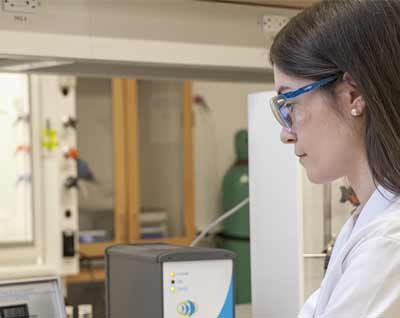
This guide is intended for owners of the AfterMath software package who use the software to control electrochemical instrumentation manufactured by Pine Research Instrumentation.

The reader is assumed to have a good working knowledge of electrochemistry (voltammetry, electrochemical cells, corrosion, etc.).

The reader is also assumed to have a operational knowledge of other non-electrochemical features of the AfterMath software package. These other features of AfterMath are described in the primary AfterMath User's Guide and they are not discussed here. The Electrochemist's Guide to AfterMath deals only with issues pertaining to the use of AfterMath with an electrochemical potentiostat/galvanostat system.

Related Links: Electrochemist's Guide, AfterMath User's Guide, AfterMath Main Support Page

Posted 1/4/2016 in Uncategorized
Read More

Koutecky-Levich Rotating Disk Electrochemistry (KL-RDE)

This article is part of the AfterMath Data Organizer Electrochemistry Guide

Koutecky-Levich Rotating Disk Electrochemistry (KL-RDE) is Rotating Disk Electrochemistry (RDE) that automatically steps through a series of rotation speeds. Currents at each rotation speed are plotted as a function of potential to obtain a series of voltammograms.

Detailed Description

Like most of the other electrochemical techniques offered by the AfterMath software, this experiment begins with an induction period. During the induction period, a set of initial conditions is applied to the electrochemical cell and the cell is allowed to equilibrate to these conditions. The default initial condition involves holding the working electrode potential at the Initial Potential for a brief period of time (i.e., 3 seconds). Since the potentiostat is being used to control the rotator speed, the rotator is also spun at the desired Initial speed during this time.

At each rotation speed, the potential of the rotating disk is cycled according to the parameters the you entered. After the sweep has finished at the final rotation speed, the experiment concludes with a relaxation period. The default condition during the relaxation period involves holding the working electrode potential at the final potential for an additional brief period of time (i.e., 1 seconds).

At the end of the relaxation period, the post experiment idle conditions are applied to the cell and the instrument returns to the idle state.

Current is plotted as a function of the potential applied to the rotating disk for each rotation speed, resulting in a series of voltammograms.

Parameter Setup

The parameters for this method are arranged on various tabs on the setup panel. The most commonly used parameters are on the Basic tab, and less commonly used parameters are on the Advanced tab. Additional tabs for Ranges and Post Experiment Conditions are common to all of the electrochemical techniques supported by the AfterMath software.

Basic Tab

You can click on the “I Feel Lucky” button (located at the top of the setup) to fill in all the parameters with typical default values. You will no doubt need to change the Initial Potential, Final Potential, and Sweep Rate to values which are appropriate for the electrochemical system being studied.

The Basic tab contains the same parameters as RDE except that the Rotator Parameters box contains an Initial speed, a Final speed, an Increment method, and an Iterations (see Figure 1). The rotation speeds will be chosen based on the Increment method and the number of Iterations. The different Increment methods are Linear, Levich, Koutecky, Eisenberg and Custom (see Figure 2). When Linear is chosen the rotation speeds will be evenly spaced between the Initial speed and Final speed. When Levich is chosen, the increments will be spaced such that the increases in the limiting current ( $i_{lim}$ ) are constant with respect to ${\omega}^{1/2}$ ( ${\Delta}i_{lim} \; {\alpha}\;{\Delta}{\omega}^{1/2})$ . When Koutecky is chosen, the increments will be spaced such that the inverse of the increases in the limiting current are constant with respect to $1/{\omega}^{1/2} (1/{\Delta}i_{lim} \; {\alpha} \; 1/{\Delta}{\omega}^{1/2})$ . When Eisenberg is chosen, the increments will be spaced such that the increase in limiting current is proportional to ${\omega}e^{0.7}$ ( ${\Delta}i_{lim} \; {\alpha} \; {\omega}e^{0.7}$ ). Finally, when Custom is chosen, you as the user enter the values of each rotation speed between the Initial speed and the Final speed.

KL-RDE is typically done in order to obtain a heterogeneous rate constant for the species of interest. Therefore, typically you choose one segment and enter an Initial potential, Final potential, Sweep rate, and Rotator Speed. Please see the webpage regarding RDE if more than one segment is needed.

Figure 1: Basic Setup Tab with Linear Increment Method Chosen.

Figure 2: Basic Setup Tab Showing Different Increment Methods.

The Electrode Range on the Basic tab is used to specify the expected range of current. If the choice of electrode range is too small, actual current may go off scale and be truncated. If the electrode range is too large, the voltammogram may have a noisy, choppy, or quantized appearance. Please see the ugly duckling webpage for more information.

Advanced Tab

The Advanced Tab for this method (see Figure 3) is the same as the Advanced Tab for RDE and allows you to change the behavior of the potentiostat during the induction period and relaxation period. By default, the potential applied to the working electrode during the induction and relaxation period will match the initial potential and final potential, respectively, as specified on the Basic Tab. You may override this default behavior, and you may also change the durations of the induction and relaxation periods if you wish.

Other important parameters on the Advanced tab are found in the Sampling Control area. This area contains two parameters, Alpha and Threshold which control when and how samples are acquired during the sweep portion of the experiment.

Figure 3: Advanced Parameters for KL-RDE

As mentioned previously, the waveform applied to the electrode (see Figure 4A for a two-segment example) is not truly linear. The actual waveform is a staircase of small potential steps (see Figure 4B). The duration of each small step is called the step period, and the step period is automatically chosen to take full advantage of the resolution of the potentiostat's digital-to-analog converter.

Figure 4: Two Segment RDE Waveform Detailing the A) Total waveform and B) Magnified Waveform Showing the Applied Potential Steps (black trace) and Measured Potential (red trace)

The Alpha parameter controls the exact time within the step period at which the current is sampled. A alpha value of zero means the current is sampled at the start of the step period, immediately after a new potential step is applied. An alpha value of 100 means the current is sampled at the end of the step period, immediately before the next potential step is applied.

Changing alpha will have little effect on the voltammogram for a freely diffusing species in solution; however, variations in alpha can dramatically influence the results for surface bound species, especially when using older potentiostats with low DAC resolution (i.e., 12-bit).

Newer potentiostats (such as the WaveNow and WaveNano portable USB potentiostats) have 16-bit DAC resolution, so voltammograms acquired using these instruments are less influenced by the choice of alpha value. Nevertheless, researchers who use digital potentiostats to study surface-confined electrochemical systems (rather than freely diffusing species in solution) should be aware of the influence of this parameter. Further details can be found in the literature¹ and in a related article about CBP Bipotentiostat Interface Boards.

The Threshold parameter helps you to limit the amount of data retained as the voltammogram is acquired. The threshold parameter controls the interval between samples as the potential is swept from one limit to another. By default, a data point is acquired every time the sweep moves 5 millivolts. You can change the threshold from 5 millivolts to a smaller interval (if you want to acquire more data) or to a greater interval (if you want to acquire less data).

Extreme values for the threshold parameter can lead to undesirable results (see Figure 7 of cyclic voltammetry). A very small Threshold value will produce smooth curves yet results in large files. A very large value though, results in jagged curves.

Ranges Tab

AfterMath has the ability to automatically select the appropriate ranges for voltage and current during an experiment. However, you can also choose to enter the voltage and current ranges for an experiment. Please see the separate discussions on autoranging and the Ranges Tab for more information.

Post Experiment Conditions Tab

After the Relaxation Period, the Post Experiment Conditions are applied to the cell. Typically, the cell is disconnected but you may also specify the conditions applied to the cell. Please see the separate discussion on post experiment conditions for more information.

Typical Results

Consider a $0.3 \; mM$ Ferrocene solution in $0.1 \; M \; Bu_4NClO_4/MeCN$ . The typical results obtained from KL-RDE are a series of sigmoid shaped voltammograms (see Figure 5, specific parameters were: rotation speeds $300-2500$ , $5$ increments, $20 \; mV/s$ sweep rate, $5 \; mM$ Pt disk).

Figure 5: KL-RDE Results for a Ferrocene Solution

You can add a peak height tool to each of the voltammograms in order to obtain limiting currents (i_lim) at each rotation speed. The example below, taken from the RDE webpage, illustrates how to determine $i_{lim}$ . Right click on the trace and select “Add Tool » Peak Height” (see Figure 6). The peak height that is initially drawn (see Figure 7) may have to be changed to properly measure $i_{lim}$ . Note, specific parameters for figures 6 and 7 were: $0.5 \; mM$ Ferrocene in $0.1 \; M \; Bu_4NClO_4/MeCN$ , $5 \; mm$ Pt disk, $500 \; rpm$ , and $20 \; mV/s$ sweep rate.

Figure 6 Adding the Peak Height Tool to Measure Limiting Current

Figure 7: Addition of Peak Height Tool to Measure Limiting Current

By dragging the control points on the tool around you can draw a proper baseline (see Figure 8).

Figure 8: A Proper Baseline for Measurement of the Limiting Current

The baseline type that is initially chosen typically does a good job for a one component reversible system such as that shown above. However, you can change the baseline type by right clicking on the tool and selecting “Properties” (see Figure 9).

Figure 9: Selection of Baseline Properties

This will bring up a dialog box where you can select the type of baseline from the drop-down menu (see Figure 10).

Figure 10: Dialog Box Showing Baseline Types

After all the limiting currents have been determined (see Figure 11) you can plot $i_{lim}$ versus ${\omega}^{1/2}$ ( $\omega$ is the rotation speed in $rad/s$ ), to check that the species of interest is freely diffusing in solution (see Figure 12). The result should be a straight line.

Figure 11: Results with Peak Heights for a Ferrocene Solution

Current versus square root of rotation speed

Figure 12: $i_{lim}$ versus ${\omega}^{1/2}$

As determined by the equation shown below, plotting $1/i_{lim}$ versus $1/{\omega}^{1/2}$ will give a plot (see Figure 13) whose y-intercept is the inverse of the limiting current as determined by the heterogeneous rate constant ( $i_{k}$ ).

$\frac{1}{i_{lim}} = \frac{1}{i_k} + \frac{1}{0.62nFAD^{2/3}{\omega}^{1/2}{\nu}^{-1/6}C}$

where $n$ is the number of electrons for the reaction, $F$ is Faraday's Constant ( $96485 \; C/mol$ ), $A$ is the electrode area (in $cm^2$ ), $D$ is the diffusion coefficient of the species of interest (in $cm^2/s$ ), ${\nu}$ is the kinematic viscosity (in $cm^2/s$ ) and $C$ is the concentration (in $mol/cm^3$ ).

Figure 13: Koutecky-Levich plot.

Theory

The theory section is split between what has already been defined for RDE in a prior webpage, and additional information about Koutecky-Levich RDE.

Rotating Disk

The following theoretical introduction to RDE is intended to give the reader a general understanding so that they may better understand what parameters affect the outcome in a typical experiment. A more detailed description can be found in Bard and Faulkner.² Rotating the electrode is a method of forced convection with the purpose of continually delivering material to the electrode in a controlled manner. The rotating rod creates a vortex flow underneath the electrode which pulls material upwards.

The purpose of rotating the electrode is to keep the solution homogeneous. However, next to the electrode is a stagnant layer, called the Levich layer which actually “clings” to the electrode and rotates with it. Inside this layer, the primary mode of mass transport is diffusion. Even though the primary mode of mass transport is diffusion like in cyclic voltammetry, linear sweep voltammetry, or chronoamperometry the concentration gradient at the electrode remains constant with respect to time. Since the concentration gradient remains constant with respect to time, the current is a steady-state current.

The thickness of the Levich layer will depend upon the experimental conditions and is governed by the equation

${\delta}_L = 1.61 D^{1/3}{\omega}^{-1/2}{\nu}^{1/6}$

where $D$ is the diffusion coefficient (in $cm^2/s$ ), $\omega$ is the rotation speed ( $rad/s$ ), and $\nu$ is the kinematic viscosity (in $cm^2/s$ , see Table 1).

Table 1: Kinematic Viscosities for $0.1 \; M \; Et_4NClO_4$ Solutions at $25^{\circ}C$ ¹
Solution	${\nu} (cm^2/s)$
$H_2O$	$0.009132$
$H_2O \; (0.1 \; M \; KCl)$	$0.008844$
$MeCN$ (acetonitrile)	$0.004536$
$DMSO$ (dimethylsulfoxide)	$0.01896$
Pyridine	$0.009518$
$DMF$ (dimethylformamide)	$0.008971$
N,N-Dimethylacetamide	$0.01067$
$HMPA$ (hexamethylphosphoramide)	$0.03530$
$D_2O$	$0.01028$

The limiting current at electrode is proportional to the thickness of the Levich layer and is defined by

$i_{lim} = nFAC\left(\frac{D}{\delta}\right)$

where $n$ is the number of electrons in the electrochemical reaction, $F$ is Faraday's constant ( $96485 \; C/mol$ ), $A$ is the electrode area (in $cm^2$ ), and $C$ is the concentration (in $mol/cm^3$ ). Finally, the fully expanded limiting current is defined by the Levich equation,

$i_{lim} = nFAD^{2/3}{\omega}^{1/2}{\nu}^{-1/6}C$ .

Koutecky-Levich RDE

The limiting current described in the section above is the diffusion limited current for RDE. KL-RDE is used to extract heterogeneous rate constants for the species of interest. This is accomplished by extrapolating what the limiting current would be at infinitely high rotation speeds. Consider the equation below

$\frac{1}{i_{lim}} = \frac{1}{i_k} + \frac{1}{0.62nFAD^{2/3}{\omega}^{1/2}{\nu}^{-1/6}C}$

where $i_k$ is the heterogeneous rate constant limited current, and the other parameters are as described above. Plotting $1/i_{lim}$ vs. $1/{\omega}^{1/2}$ will give a line whose y-intercept is $1/i_k$ . The heterogeneous rate constant can be calculated using the equation

$i_k = nFAk^oC$

where $k^o$ is the heterogeneous rate constant (in $cm/s$ ) and the other parameters are as above.

Application

In the first example, Rajasekharan et al.³ use KL-RDE to extract heterogeneous rate constants for for the reduction of free chlorine and monochloramine. Studying these two chlorines is significant because they are the most commonly used drinking water disinfectants. The researchers found that the reduction of free chlorine proceeds twice as fast as monochloramine.

The second example Finklestein et al.⁴ use KL-RDE to investigate the oxidation of $BH_4^-$ at gold and platinum surfaces. The researchers studied these two surfaces due to possible use in a borohydride fuel cell. Conventional wisdom has been that gold will outperform platinum in a $BH_4^-$ fuel cell, however, by using KL-RDE the researchers were able to show that platinum is a more ideal surface for the oxidation of $BH_4^-$ due to higher heterogeneous rate constants and also a larger operational window.

The third example uses KL-RDE in a slightly different way. Rather than measuring heterogeneous rate constants, Shigehara et al.⁵ used KL-RDE to investigate self-exchange rates for $IrCl_6^{2-/3-}$ and $Fe(CN)_6^{3-/4-}$ . Polyelectrolytes were initially deposited on the electrode surface followed by electrostatic self assembly of the redox species of interest. Using KL-RDE allowed the researchers to extract the self-exchange rate constant since the limiting step at infinitely high rotation rates would be the exchange of the electrons between complexes at the film/solution interface.

In the final example, Kundu et al.⁶ used KL-RDE to investigate the oxygen reduction reaction (ORR) using doped and undoped carbon nanotubes. Rather than extracting a rate constant the researchers used the slope of the Koutecky-Levich plot to obtain the number of electrons transferred during the ORR. Using doped carbon nanotubes, the researchers found that the number of electrons transferred during the reaction was 4, meaning that oxygen is reduced to $H_2O$ in a four electron process. Using undoped carbon nanotubes, the researchers found that the number of electrons transferred was 2.5, meaning that most of the oxygen in this case is reduced to $H_2O_2$ .

References

1. He, P. Anal. Chem., 1995, 67, 986-992.

2. Faulkner, L. R.; Bard, A. J. Potential Sweep Methods, Electrochemical Methods: Fundamentals and Applications, 2^nd ed.; Wiley: New Jersey, 2000; 226-260.

3. Rajasekharan, V. V.; Clark, B. N.; Boonsalee, S.; Switzer, J. A. Environ. Sci. Technol., 2007, 41, 4252–4257.

4. Finklestein, D. A.; Da Mota, N.; Cohen, J. L.; Abruna, H. D. J. Phys. Chem. C., ASAP

5. Shigehara, K.; Oyama, N.; Anson, F. C. Inorg. Chem., 1981, 20, 518-522.

6. Kundu, S.; Nagaiah, T. C.; Xia, W.; Wang, Y.; Von Dommelle, S.; Bitter, J. H.; Santa, M.; Grundmeier, G.; Bron, M.; Schuhmann, W.; Muhler, M. J. Phys. Chem. C, 2009, 113, 14302–14310.

Additional Resources

Links: Electrochemist's Guide, AfterMath User's Guide, AfterMath Main Support Page

Posted 1/4/2016 in Uncategorized

Linear Sweep Voltammetry (LSV)

This article is part of the AfterMath Data Organizer Electrochemistry Guide

Linear sweep voltammetry involves scanning the potential of the working electrode linearly with time at rates typically between 10 mV/s and 1000 V/s. The current is plotted as a function to potential to yield a voltammogram.

Synonyms: Linear potential sweep chronoamperometry

Detailed Description

Linear sweep voltammetry is simply cyclic voltammetry without a Vertex Potential and reverse scan. Users are referred to the description on Cyclic voltammetry for more detail regarding instrument setup and acquisition. The basic setup will be discussed here. The setup panel for linear sweep voltammetry is as shown in Figure 1. The user can choose an Initial potential, Final potential and Sweep rate. Electrode range can be Auto or chosen by the user provided the range of currents for the experiments are known.

Figure 1: Basic setup for linear sweep voltammetry.

The Advanced, Ranges, and Post Experiment Conditions tabs are identical in setup to the Cyclic voltammetry tabs. Finally, a plot of the potential applied to the electrode is shown in Figure 2. Note that the flat portions at the beginning of the scan and the end of the scan are the Induction period and Relaxation periods, respectively. Details regarding these two periods are provided in separate wikis. After completion of the experiment and relaxation period, the post experiment idle conditions are applied to the cell.

Figure 2: Applied potential for linear sweep voltammetry.

Theory and Application

The user is referred to the section on Cyclic voltammetry for a discussion on theory.

Most applications of linear sweep voltammetry relate to cyclic voltammetry. However, here are a few examples where linear sweep voltammetry was applied.

In the first example,¹ Cheng and coworkers used linear sweep voltammetry to examine direct methane production using a biocathode containing methanogens in either an electrochemical system or a microbial electrolysis cell by a process called electromethanogenesis. Since the production of methane from $CO_2$ is an irreversible process, cyclic voltammetry would provide no additional benefit over linear sweep voltammetry. Linear sweep voltammetry was used to show that a biocathode produced higher current densities than a plain carbon cathode. The authors were able to show that methane can be produced directly from an electrical current without hydrogen gas.

In another example,² Wang and coworkers used linear sweep voltammetry to examine the release of inorganic ions and DNA from an ionorganic ion/DNA bilayer film. Performing linear sweep voltammetry simultaneously with surface plasmon resonance, the researchers were able to show that the film disassembled upon sweeping the potential to more negative values. This allowed the researchers to demonstrate the controlled release of DNA for gene-targeting therapy.

References

1. Cheng, S.; Xing, D.; Call, D. F.; Logan, B. E. Environ. Sci. Technol., 2009, 43, 3953–3958.

2. Wang, F.; Li, D.; Li, G.; Liu X.; Dong, S. Biomacromolecules, 2008, 9, 2645–2652

Additional Resources

Links: Electrochemist's Guide, AfterMath User's Guide, AfterMath Main Support Page

Related Techniques: Cyclic Voltammetry (CV), Staircase Voltammetry (SCV)

Posted 1/4/2016 in Uncategorized
Read More
Double Potential Step Chronoamperometry (DPSCA)

This article is part of the AfterMath Data Organizer Electrochemistry Guide

Double potential step chronoamperometry is a technique where the potential of the working electrode is stepped forward for a specified period of time, then stepped back for a specified period of time. Current is monitored and plotted as a function of time.

Detailed Description

Like most of the other electrochemical techniques offered by the AfterMath software, this experiment begins with an induction period. During the induction period, a set of initial conditions is applied to the electrochemical cell and the cell is allowed to equilibrate to these conditions. The default initial condition involves holding the working electrode potential at the Initial Potential for a brief period of time (i.e., 3 seconds).

After the induction period, the potential of the working electrode is stepped to a specified potential for a period of time.

After the first step has finished, the potential of the working electrode is stepped back for a specified period of time, usually to the potential prior to the forward step. The experiment concludes with a relaxation period. The default condition during the relaxation period involves holding the working electrode potential at the initial potential for an additional brief period of time (i.e., 1 seconds).

At the end of the relaxation period, the post experiment idle conditions are applied to the cell and the instrument returns to the idle state.

Current is plotted as a function of time, resulting in a chronoamperogram. You may also choose to do some post experiment processing in order to generate Cottrell plots.

Parameter Setup

The parameters for this method are arranged on various tabs on the setup panel. The most commonly used parameters are on the Basic tab which is similar to that for CA with the addition of a Reverse step period box. Additional tabs for Ranges and Post Experiment Conditions are common to all of the electrochemical techniques supported by the AfterMath software. Finally, a Post Experiment Processing tab deals with manipulating the data automatically when the experiment is finished.

Basic Tab

You can click on the “I Feel Lucky” button (located at the top of the setup) to fill in all the parameters with typical default values (see Figure 1). You will no doubt need to change the Potential and Hold time in the Forward step period and Reverse step period boxes to values which are appropriate for the electrochemical system being studied. You may also want to change the Number of intervals in the Sampling Control box.

Figure 1: Basic Setup for Double Potential Step Chronoamperometry.

The Electrode K1 Current Range on the Basic tab is used to specify the expected range of current. If the choice of electrode range is too small, actual current may go off scale and be truncated. If the electrode range is too large, the chronoamperogram may have a noisy, choppy, or quantized appearance.

Some Pine potentiostats (such as the WaveNow and WaveNano portable USB potentiostats) have current autoranging capability. To take advantage of this feature, set the electrode range parameter to “Auto”. This allows the potentiostat to choose the current range “on-the-fly” while the chonoamperogram is being acquired.

The waveform that is applied to the electrode is a simple pulse to the Potential listed in the Forward step period box for the Hold time followed by a step back to the Potential specified in the Reverse step period box. Note that the actual waveform that is measured (see Figure 2, red trace) fluctuates slightly compared to the applied potential (see Figure 2, black trace).

Figure 2: Waveform for DPSCA. Black = applied potential, Red trace = measured potential.

Ranges Tab

AfterMath has the ability to automatically select the appropriate ranges for voltage and current during an experiment. However, you can also choose to enter the voltage and current ranges for an experiment. Please see the separate discussions on autoranging and the Ranges Tab for more information.

Post Experiment Conditions Tab

After the Relaxation Period, the Post Experiment Conditions are applied to the cell. Typically, the cell is disconnected but you may also specify the conditions applied to the cell. Please see the separate discussion on post experiment conditions for more information.

Post Experiment Processing Tab

The Post Experiment Processing Tab (see Figure 3) looks similar to that for CA and allows you to automatically generate Cottrell current, Cottrell charge, DPSCA working curve, or DPSCC working curve plots. Please see the Typical Results and Theory sections of this wiki for more information regarding Cottrell plots and DPSCA/DPSCC working curves.

Figure 3: Post Experiment Processing Options.

Typical Results

The results for a $2.5 \; mM$ solution of Ferrocene in $0.1 \; M Bu_4NClO_4/MeCN$ are shown in Figure 4. Specific conditions include the use of a $2 \; mm$ Pt WE, forward step potential of $0.75 \; V \; vs. \; Ag/AgCl_{(aq)}$ and reverse step potential of $0 \; V \; vs. \; Ag/AgCl_{(aq)}$ .

Figure 4: Double Potential Step Chronoamperogram of a Ferrocene Solution

If you selected to automatically generate Cottrell plots, the plots are under the other plots folder in the Archive navigation panel. Choosing Cottrell current displays a plot of current versus the $t^{-1/2}$ (see Figure 5A). Choosing Cottrell charge displays a plot of charge versus $t^{1/2}$ (see Figure 5B). Note that for the Cottrell Current plot, the level portion in the plot is actually the time prior to the current spike shown in Figure 4. That is, earlier time points are to the right in a Cottrell Current Plot. This is not the case for a Cottrell Charge plot because integrating the current with respect to time gives charge.

Figure 5 : Post experiment processing plots. A – Cottrell Current, B – Cottrell Charge. Conditions as listed in Figure 4.

If you selected to automatically generate DPSCA or DPSCC working curves, they are also under the other plots folder in the Archive navigation panel. The theory for the forward step in DPSCA is the same as the theory for the first step in CA, however the theory for the reverse step is complicated by the first step. The DPSCA working curve (see Figure 6) is a useful way to examine if kinetic complications of the redox species are present. If there are no kinetic complications and both potential steps are to regions of diffusion-limited currents, the actual (see Figure 6, red trace) working curve will overlay the ideal (see Figure 6, black trace) working curve. The ideal working curve is theoretically generated according to the equation

${\frac{-i_r}{i_f}}= 1 - \left(1-\frac{\tau}{t_r}\right)^{1/2}$

where $i_r$ is the reverse current at $t_r$ , $i_f$ is the forward current at $t_f$ and $\tau = t_r-t_f$ . A quick check for a stable system is:

$\frac{-i_r(2\tau)}{i_f(\tau)}=0.293$

Figure 6: DPSCA Working Curve. Actual = red trace, Ideal = black trace. Conditions as listed in Figure 4.

The DPSCC working curve (see Figure 7) is a useful way to examine the charge passed during an experiment and is similar to the Cottrell Charge plot except that it separates the forward (see Figure 7, red trace) and reverse (see Figure 7, black trace) steps. The reverse step is corrected to account for the charge passed during the forward step, making the charge passed in the reverse step linear with respect to time.

Figure 7 : DPSCC Working Curve. Forward – red trace, Reverse – black trace. Conditions as listed in Figure 4.

Theory

As stated in the Theory section of CA, the time-dependent current transient in a diffusion-limited chronoamperometry experiment is governed by the Cottrell² equation

$i=\frac{nFAD^{1/2}C_0^*}{({\pi}t)^{1/2}}$

where $n$ is the number of electrons, $F$ is Faraday's Constant ( $96485 \; C/mol$ ), $A$ is the electrode area ( $cm^2$ ), $D$ is the diffusion coefficient ( $cm^2/s$ ), and $C$ is the concentration ( $mol/cm^3$ ). In DPSCA, the time of the transition must be taken into account. The current transient for the second pulse, provided it produces diffusion-limited currents, is governed by the equation first obtained by Kambara³

$-i_r(t) = \frac{nFAD_0^{1/2}C_0^*}{\pi^{1/2}}\left[\frac{1}{(t-\tau)^{1/2}}-\frac{1}{t^{1/2}}\right]$

where $\tau$ is the transition time and the other parameters are as above. Dividing the reverse current at time $t_r$ by $i_f [latex] at time [latex] t_f$ and keeping $t_r = t_f + \tau$ allows for the generation of a working curve given by the equation

$\frac{-i_r}{i_f} = 1-\left(1-\frac{\tau}{t_r}\right)^{1/2}$

If there are no kinetic complications in the electrode reaction, the actually working curve should fall on an ideal working curve as shown in Figure 6. Note that the deviation at the beginning of the working curve is due to the electronics of the potentiostat.

DPSCA is a technique that is often used to elucidate mechanisms related to coupled homogeneous reactions preceeding or following an electrode reaction. Bard and Faulkner¹ give a more detailed description of using DPSCA to elucidate mechanisms. A brief description will be given here as to what types of mechanisms can be elucidated and how you might apply DPSCA. Several examples are listed in the Application section also.

The simplest coupled homogeneous reactions are Electrochemical-Chemical (EC) and Chemical-Electrochemical (CE).

Application

This example uses DPSCA to calculate the diffusion coefficients for a subtrate ( $D _s$ ) and a product ( $D_p$ ) of an electrode reaction. Hyk et al.⁴ examined the current transients for DPSCA to analyze the reaction $S_s^Z \rightarrow P_p^Z + ne^-$ . The researchers generated equations for dealing with both hemispherical electrodes and disk microelectrodes under diffusion-limited and mixed diffusion-migration. Interestingly, the researchers were able to show that for an uncharged substrate with less than $0.1%$ supporting electrolyte they are able to obtain diffusion coefficients. This is significant because an uncharged substrate with less than 0.1% supporting electrolyte does not lend to calculation of diffusion coefficients by single potential step chronoamperometry.

In this next example, Long et al.⁵ used a slight variant of DPSCA to examine diffusion and self-exchange in a cobalt bipyridine redox polyether hybrid. Films of material, containing supporting electrolyte, were prepared on inter-digitated array electrodes (IDAs). A pulse was generated (equivalent to a double-potential step) on one set of fingers on the IDA while the current was monitored on the second set of fingers on the IDA. Monitoring the time it takes for the pulse to travel from the generator set of fingers to the collector set of fingers allowed for the calculation of diffusion coefficients and self-exchange rate constants between metal centers.

In the final example, Schwarz and Shain⁶ used DPSCA to measure the rate constant for a chemical reaction after an electrochemical reaction, commonly referred to as an EC reaction. The overall reaction for the general process is

$O+e^-\rightarrow R \xrightarrow{k} Z$

where the product $Z$ is electrochemically inactive. In this example, the researchers reduce azobenzene to hydrazobenzene which in turn rearranges to benzidine in acidic solutions. By varying the time of the second step, the researchers were able to determine the rate constant for the reaction of hydrazobenzene rearrangning to benzidine.

References

1. Faulkner, L. R.; Bard, A. J. Basic Potential Step Methods, Electrochemical Methods: Fundamentals and Applications, 2^nd ed.; Wiley: New Jersey, 2000; 156-225.

2. Cottrell, F. G. Z. Physik, Chem., 42, 1902, 385.

3. Kambara, T. Bull. Chem. Soc. Jpn., 1954, 27, 523.

4. Hyk, W; Nowicka, A.; Stojek, Z. Anal. Chem., 2002, 74, pp 149–157.

5. Long, J. W.; Terrill, R. H.; Williams, M. E.; Murray, R. W. Anal. Chem., 1997, 69, pp 5082–5086.

6. Schwarz, W. M.; Shain, I. J. Phys. Chem., 1965, 69, pp 30-40.

Additional Resources

Links: Electrochemist's Guide, AfterMath User's Guide, AfterMath Main Support Page

Related Techniques: Chronoamperometry (CA)

Posted 1/4/2016 in Uncategorized
Read More

previous 10

Next 10

	$n{\Delta}E_i/mV$
$n{\Delta}E_a/mV$	$1$	$5$	$10$	$20$
$0^b$	$0.0053$	$0.0238$	$0.0437$	$0.0774$
$10$	$0.2376$	$0.2549$	$0.2726$	$0.2998$
$20$	$0.4531$	$0.4686$	$0.4845$	$0.5077$
$50$	$0.9098$	$0.9186$	$0.9281$	$0.9432$
$100$	$1.1619$	$1.1643$	$1.1675$	$1.1745$