WaveDriver Dual Channel (K1 and K2) DC Test

Last Updated: 1/9/23 by Alex Peroff

ARTICLE TAGS

DC test,
WaveDriver test,
dual channel,
2 channel test,
two channel test

Related Products

Related AfterMath Entries

AfterMath Downloads

Article Contents/Section Navigation

WaveDriver Dual Channel (K1 and K2) DC Test

1WaveDriver Dual Channel (K1 and K2) DC Test

This test is performed during the system testing of a Pine Research WaveDriver potentiostat (WaveDriver 200 and WaveDriver 40 models).

1.1Connect to WaveDriver Dummy Cell

Securely connect the cell cable to the front panel of the WaveDriver (see Figure 1 for examples for each WaveDriver model). Remove any alligator clips from the banana plugs and insert the plugs into the banana jacks with matching colors for each lead on Row “C” of the dummy cell that accompanies the specific model of WaveDriver (for the WaveDriver 200, it is the EIS Calibration & Dummy Cell; for the WaveDriver 40, it is the Universal Dummy Cell).

Be sure to also connect the GRAY banana plug (instrument chassis) to the chassis terminal located on the dummy cell. Connecting the two chassis terminals together effectively shields the instrument circuitry and the components of the dummy cell within the same overall Faraday cage.

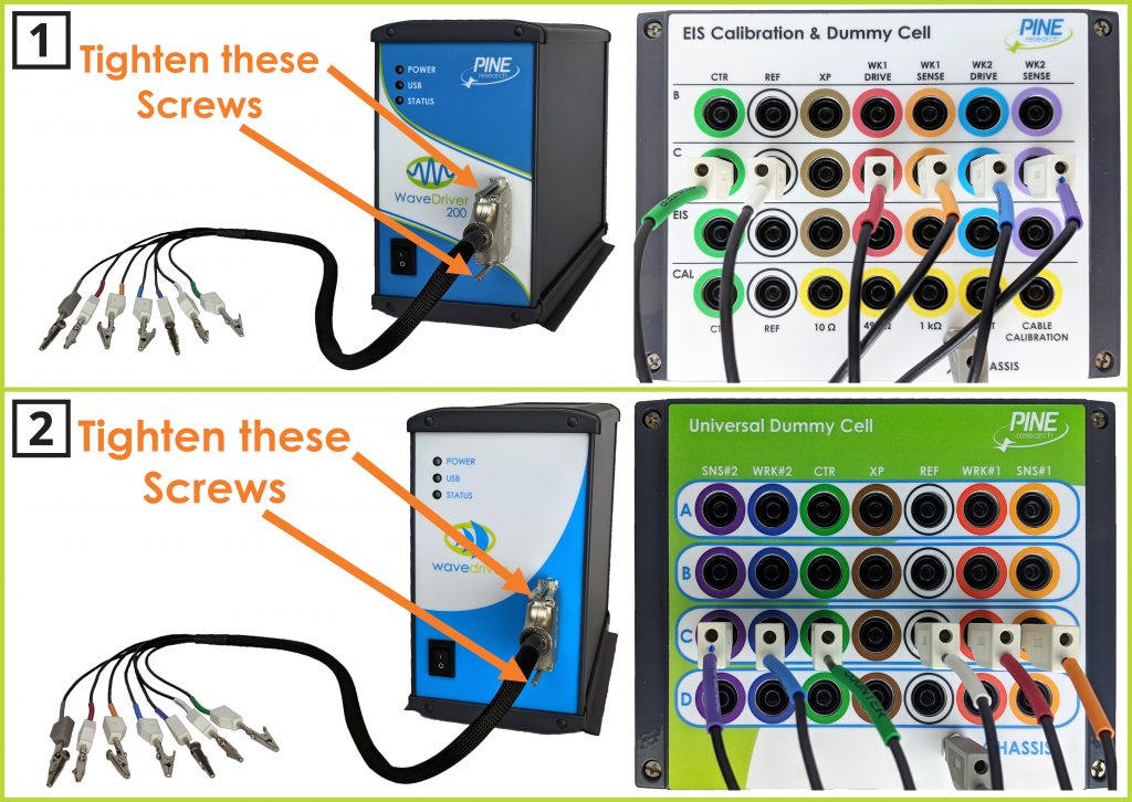
WaveDriver Cell Cable Connected to Dummy Cell Row “C”

Figure 1. Cell Cable Connected to Dummy Cell Row “C” for (1) WaveDriver 200; and (2) WaveDriver 40

1.2Create a Dual Electrode Cyclic Voltammetry (DECV) Experiment

Choose the Dual Electrode Cyclic Voltammetry (DECV) option from the Dual electrode methods sub-menu in the AfterMath Experiments menu. A new DECV specification will be created and placed into a new archive. Configure the parameters as detailed below (see Figure 2).

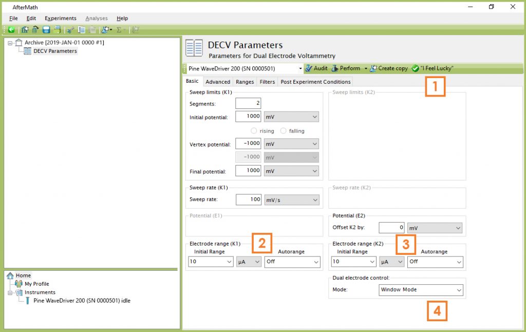
1	Click on the “I Feel Lucky” button. Note that default parameters for number of Segments, Sweep limits, and Sweep rate appear automatically.
2	Set the Electrode range (K1) to “10 µA” with Autorange “Off”
3	Set the Electrode range (K2) to “10 µA” with Autorange “Off”
4	Change the Dual electrode control mode to “Window Mode”

Figure 2. Dual Electrode Cyclic Voltammetry (DECV) Parameters Dialog Window

TIP: The "I Feel Lucky" button has been renamed "AutoFill" in versions of AfterMath later than May 2019. Newer versions may appear with this change in terminology; however, the functionality of the button remains the same.

1.3Modify the Potential Range Setting

Select the 2.5 V range for both working electrodes (K1 and K2) via the following steps:

Click the “Ranges” tab (see Figure 3).
Change the potential electrode range for both K1 and K2 to 2.5 V and set Autorange to “Off”.

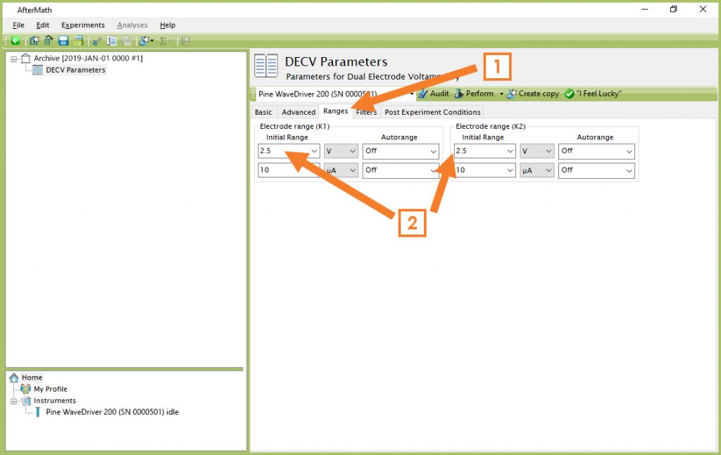
Figure 2. Adjusting the Potential Ranges on the “Ranges” Tab (DECV)

1.4Audit Experimental Parameters

Choose the WaveDriver instrument in the drop-down menu (see Figure 3, to the left of the “Audit” button), and then press the “Audit” button to check the parameters. AfterMath will perform a quick audit of the parameters to ensure that all parameters are specified and within allowed ranges.

1.5Initiate the Experiment

Click the “Perform” button to initiate the DECV experiment. The “Perform” button is located just to the right of the “Audit” button (see Figure 3). If this step is not possible, consult the AfterMath Installation Guide and permissions files verification step, or contact Pine Research directly.

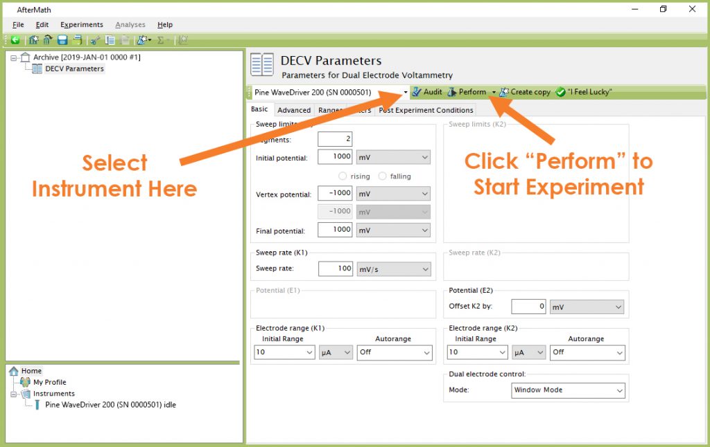
Figure 3. Location of Instrument Selection Menu and Perform Button (DECV)

NOTE: If the “Perform” button is disabled (shaded gray), this is an indication that the AfterMath software on the computer is not licensed to control the instrument. The remedy for this issue is to obtain and install the appropriate permissions files.

1.6Monitor Experimental Progress

Monitor the progress of the experiment by observing the real time plot, the percentage complete value, and the progress bar (see Figure 4).

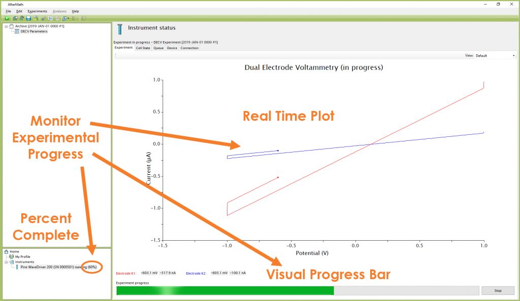
Figure 4. Monitoring the Progress of the DECV Experiment (K1 and K2)

1.7Review the Results

When the experiment is complete, the results of the experiment are placed in a folder within the archive (see Figure 5). In addition to the main voltammogram plot, additional graphs are available in the “Other Plots” folder. The results can also be viewed in tabular form under the “experiment” node.

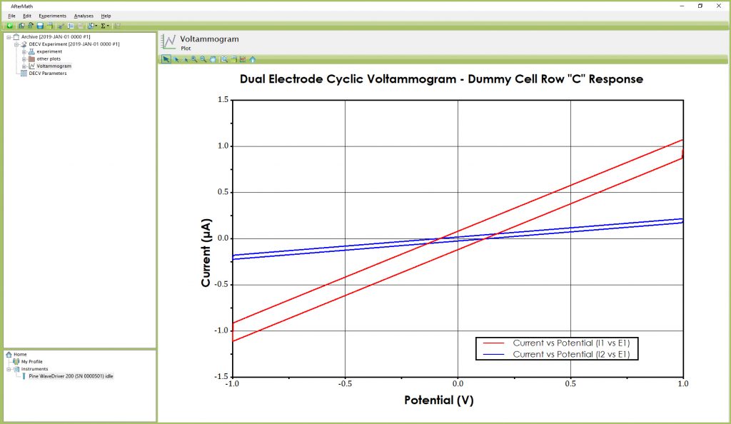
Figure 5. Anticipated DECV Results (using Dummy Cell Row “C")

EXPECTED RESULT: The anticipated test results are two diagonally-slanted parallelograms with different slopes (see Figure 5). The slope of the red trace is inversely proportional to the resistance sensed by first working electrode (~1.002 MΩ), and the slope of the blue trace is inversely proportional to the resistance sensed by the second working electrode (~5.005 MΩ). The vertical separation between sweep segments is related to the capacitance sensed by the both working electrodes (see Section 1.8).

1.8Understanding the Results

Analysis of the DECV results is similar to the analysis of the single channel WaveDriver CV test, except there are two voltammograms instead of one (see Figure 5). The red voltammogram corresponds to the first working electrode (K1) and the blue voltammogram corresponds to the second working electrode (K2).

AfterMath software baseline tools may be used to measure the slopes of the two voltammograms. To measure the slope, right-click on the desired cyclic voltammogram trace, and then select the “Baseline” option from the “Add Tool” sub-menu. A baseline measurement tool appears on the voltammogram (see Figure 6), and by adjusting the tool control points, the slope along any portion of the voltammogram can be measured.

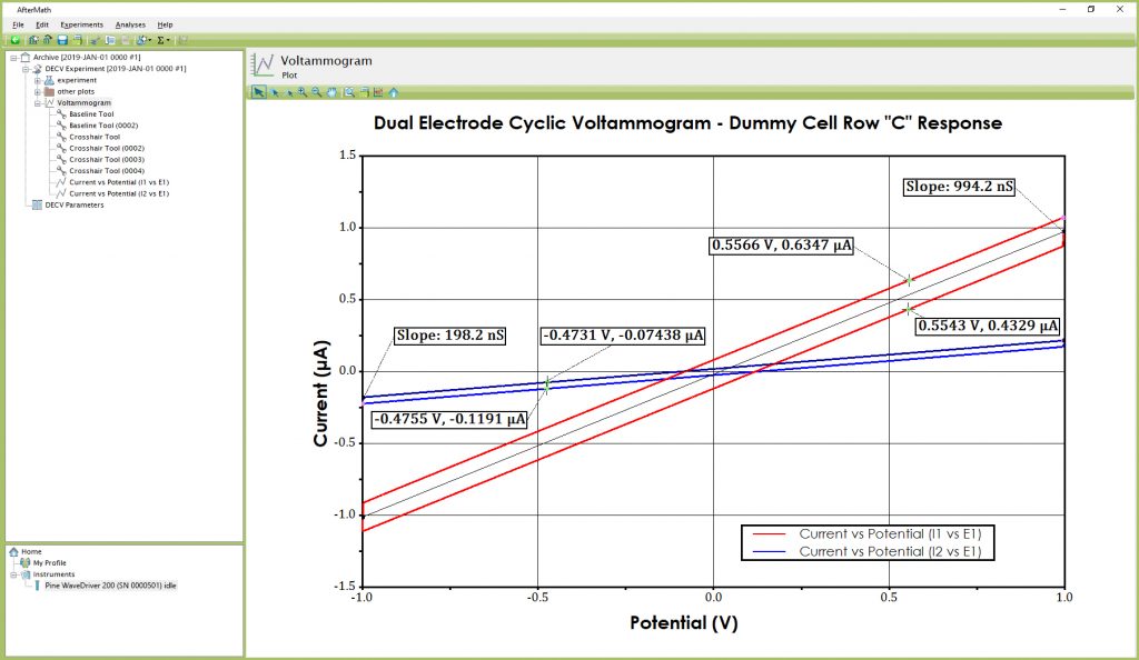
Figure 6. Analyzed DECV Results (using Dummy Cell Row “C”)

The total resistive loads sensed by both working electrodes are two separate series combinations of two resistors each: 1 MΩ + 2 kΩ = 1.002 MΩ (for K1) and 4.99 MΩ + 5 kΩ = 4.995 MΩ (for K2) (see Figure 1 in Section 1.1 of the WaveDriver Dummy Cell Descriptions). The voltammograms are plots of current vs. potential governed by Ohm’s Law, as shown in Equation 1:

$E=iR\;\;\text{(Ohm's Law)}$

(1)

where $E$ is the potential, $i$ is the current, and $R$ is the resistive load. Considering that cyclic voltammograms (see Figure 5) plot current along the vertical axis and potential along the horizontal axis, the slope $\left(i/E\right)$ is equal to the reciprocal of the resistive load (for K1, $1/R=1/1.002\;\text{M}\Omega=998\;\text{nS}$ ; for K2, $1/R=1/4.995\;\text{M}\Omega=200\;\text{nS}$ )

In the example shown here (see Figure 6), the slope for the first voltammogram (K1) is calculated as 994.2 nS, and the slope for the second voltammogram (K2) is calculated as 198.2 nS. The reciprocals of these two slopes (1.006 MΩ for K1 and 5.045 MΩ for K2) are in good agreement with the previously-mentioned resistive loads.

The nominal capacitive loads presented to the working electrodes by the dummy cell are 1 µF (for K1) and 220 nF (for K2) (see Figure 1 in Section 1.1 of the WaveDriver Dummy Cell Descriptions). The vertical separation observed between the forward and reverse segments at any point along the voltammogram is related to this capacitance. This capacitance is meant to mimic the double-layer capacitance, $C_{DL}$ , observed at the surface of an actual electrode.

Whenever a potential sweep is applied across a capacitive load, a charging current is observed. In the context of the electrode double-layer concept, the double-layer charging current, $i_{DL}$ , is related to the potential sweep rate, $\upsilon$ , and the double-layer capacitance, $C_{DL}$ , by the following equation:

$i_{DL}=C_{DL}\upsilon$

(2)

A cyclic voltammogram across a capacitor consists of a forward (i.e., charging) segment and a reverse (i.e., discharging) segment. The vertical separation between the two segments at any point along the voltammogram is two times the capacitive charging current.

To measure this vertical separation in AfterMath, right-click on the voltammogram trace and select the “Crosshair” option from the “Add Tool” sub-menu. Drag the crosshair cursor to any point on the upper segment of the voltammogram and make note of the current and potential at that point (see Figure 6). Next, create a second crosshair tool and drag it to the lower segment of the voltammogram. Position the second crosshair at the same (or nearly the same) potential as the first crosshair tool and make a note of the current and potential at that point.

Half the difference between the currents measured at the two crosshair points is the charging current. For the example shown here (see Figure 6), half the difference in current between the two points for K1 is calculated as 0.1009 µA, and for K2 it is calculated as 0.02236 µA. With knowledge of the potential sweep rate (100 mV/s), the capacitive loads can be calculated as 1.009 µF for K1 and 223.6 nF for K2, which are in good agreement with the nominal capacitances mentioned above.

EXPLORE ADDITIONAL EXPERIMENTAL RESULTS: Archive nodes often have a “+” sign next to the node name. Click on this “+” sign to open the node. In addition to the main plot produced by an experiment, additional results can be found in the “Experiment” node and in the “Other Plots” node. Nodes may be renamed and organized in folders as desired.

How can we help? What do you want to learn? Search our knowledgebase.

Potentiostat Diagnostic Tests