


Analysis
Last Updated: 10/7/19 by Neil Spinner
1Analysis
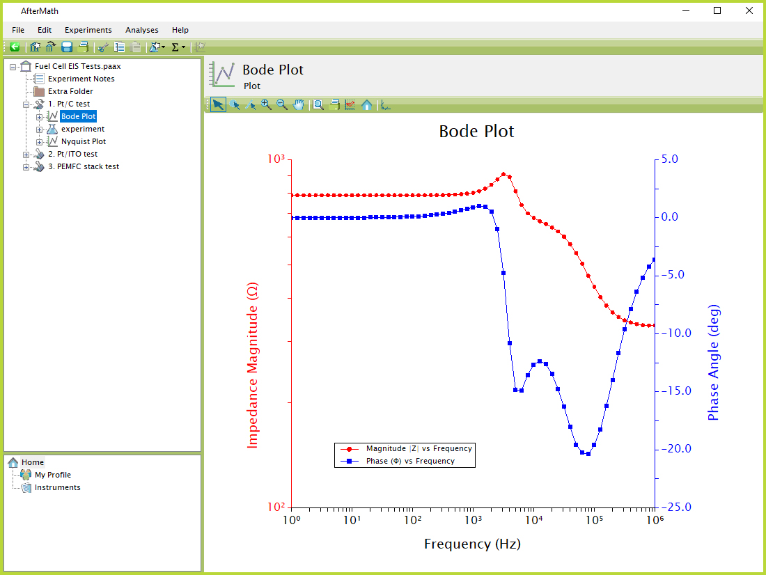
Figure 1. AfterMath Example EIS Data
There are three ways to add a new analysis node. First, with any part of an EIS data study folder
 Study
highlighted in the left tree structure, click the "Σ" symbol to open the drop-down menu of available analysis nodes (see Figure 2). The second option is the "Analyses" menu, which also opens a drop-down containing the same set of options.
Study
highlighted in the left tree structure, click the "Σ" symbol to open the drop-down menu of available analysis nodes (see Figure 2). The second option is the "Analyses" menu, which also opens a drop-down containing the same set of options.
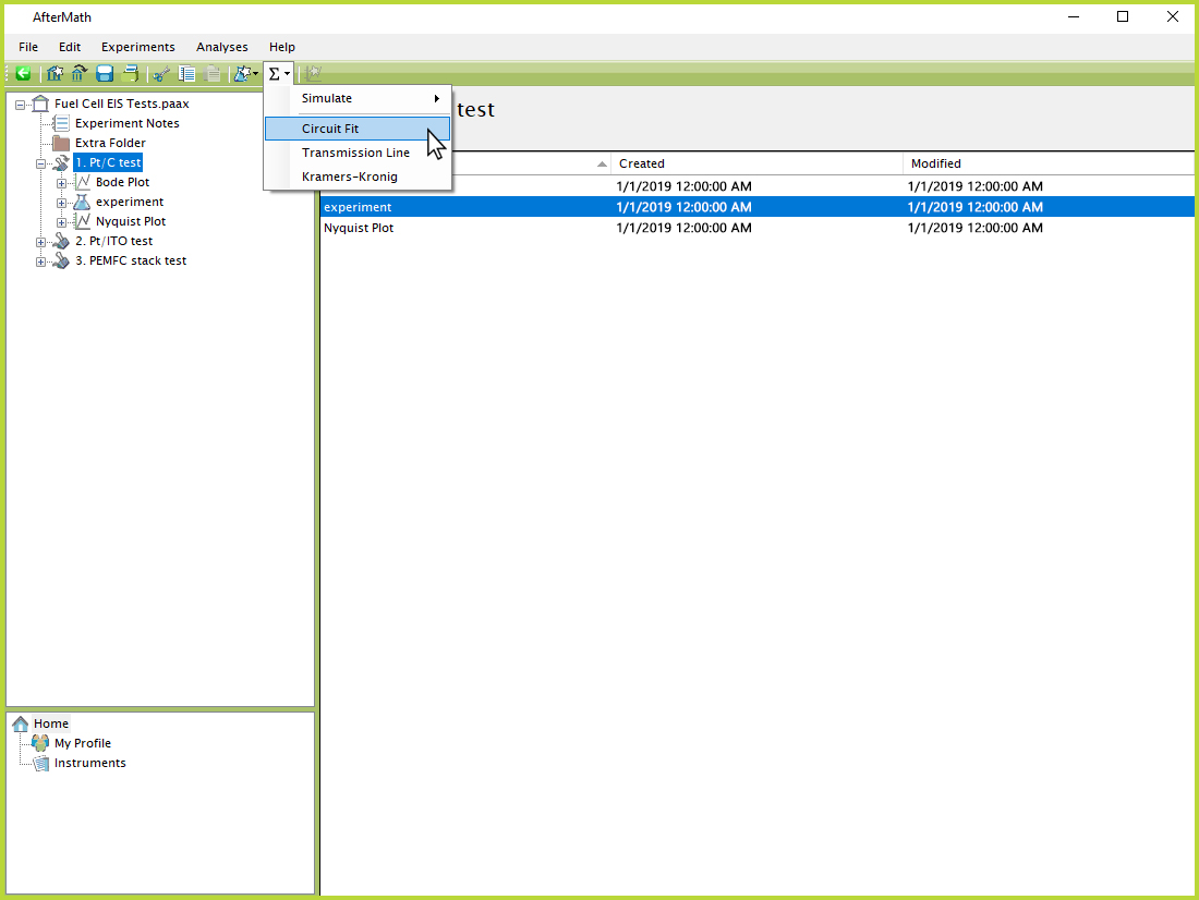
Figure 2. AfterMath Adding Analysis From Sigma Menu
Alternatively, the third option is to right-click on any part of an EIS data study folder, then select "New" from the resulting menu and click "Analysis" to reveal the set of options (see Figure 3).
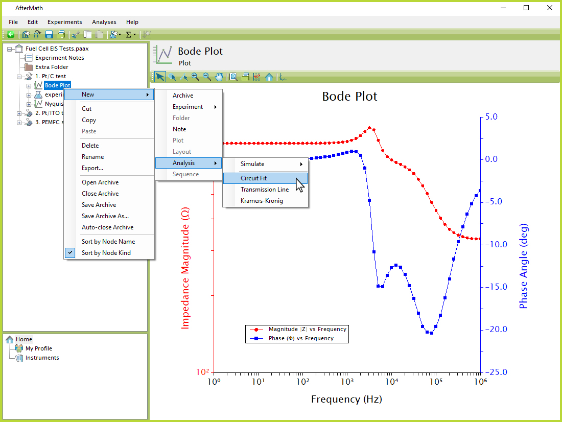
Figure 3. AfterMath Adding New Analysis Via Right-Click
The most commonly-used analysis is called "Circuit Fit", which is used to mathematically fit experimental EIS data to various circuit analogs. The first window that appears when selecting "Circuit Fit" from the list of analysis options is the "Circuit Library" (see Figure 4). This window displays a set of built-in circuit models to choose from, as well as the option for the user to construct a custom circuit by double-clicking "New..." under the "User-Defined Circuits" section. Clicking this option opens a separate designer window where a custom circuit can be drawn to fit to the experimental data, and also saved as a template for future use (see Figure 5).
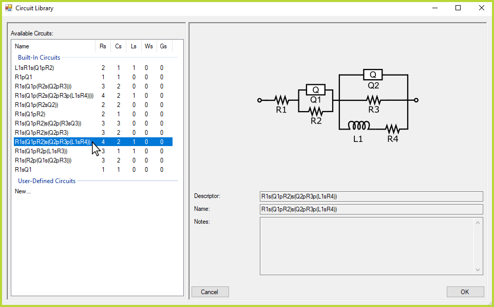
Figure 4. AfterMath Circuit Library Window
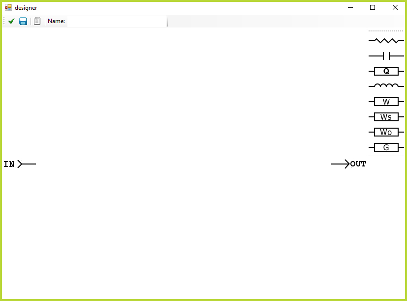
Figure 5. AfterMath Custom Circuit Designer
Once the desired circuit has been selected, AfterMath automatically performs a mathematical fitting operation on the EIS data and displays the results in the circuit fit node. Fitting data are shown both numerically for each circuit parameter, as well as graphically on the adjacent Bode
 Bode Plot
and Nyquist plots (see Figure 6).
Nyquist Plot
These two plots can also be adjusted by using the drop-down menus above each plot labeled "View". Residual error plots for the real and imaginary impedance can be viewed while adjusting the circuit fit if desired (see Figure 7).
Bode Plot
and Nyquist plots (see Figure 6).
Nyquist Plot
These two plots can also be adjusted by using the drop-down menus above each plot labeled "View". Residual error plots for the real and imaginary impedance can be viewed while adjusting the circuit fit if desired (see Figure 7).
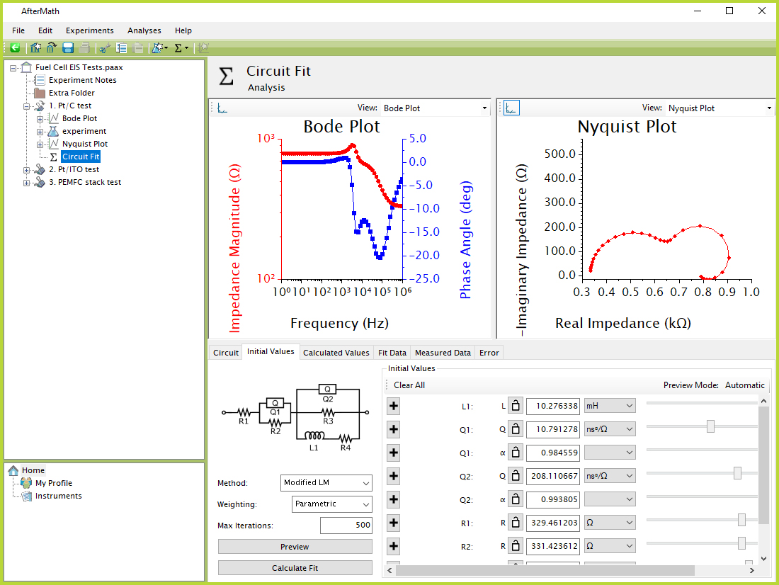
Figure 6. AfterMath Example Circuit Fit Analysis
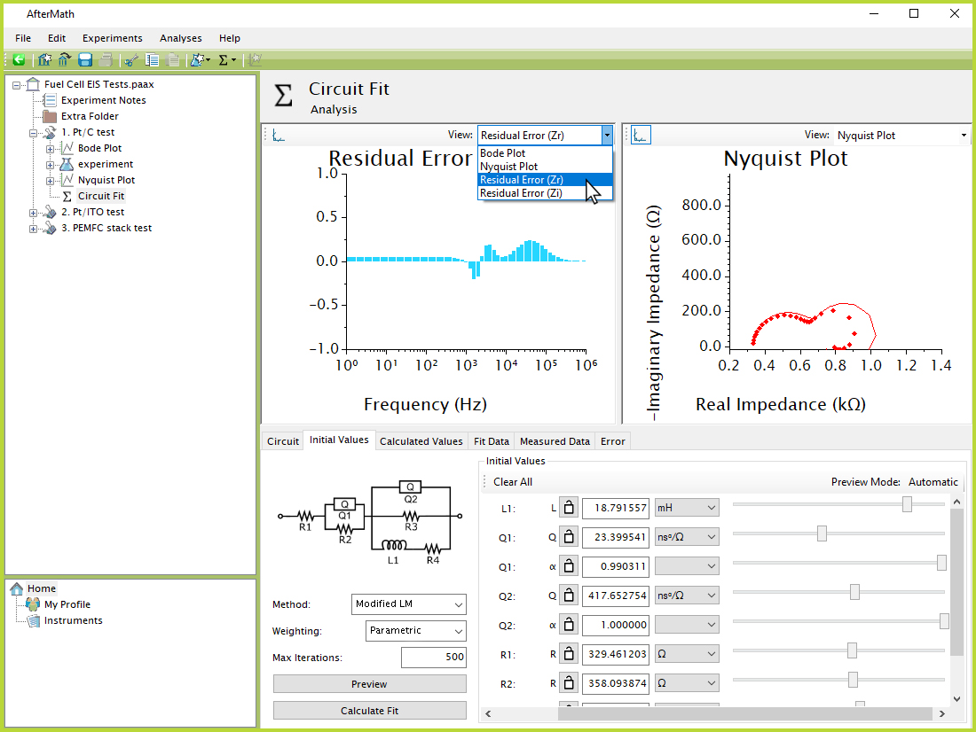
Figure 7. AfterMath Changing Plot View in Circuit Fit
Within the circuit fit node are numerous options for adjusting and/or improving the fit, in addition to different statistical analyses that can be evaluated or exported to another program if desired. These options and practices are beyond the scope of this article, and information may be found in separate posts the Pine Research Knowledgebase.
The second analysis type is called "Transmission Line", and it behaves similarly to the circuit fit analysis. After the transmission line node has been added to EIS data, the framework of a transmission line circuit appears where each element can be changed as needed using the drop-down boxes to the right of the screen under "Configuration" (see Figure 8). There are a few different preset options to choose from, or the user may specify a custom set of circuit elements to build any desired transmission line. Once the circuit has been finalized, the transmission line can be mathematically fitted to the experimental data similarly to a circuit fit. More information on transmission line can be found elsewhere on this Knowledgebase.
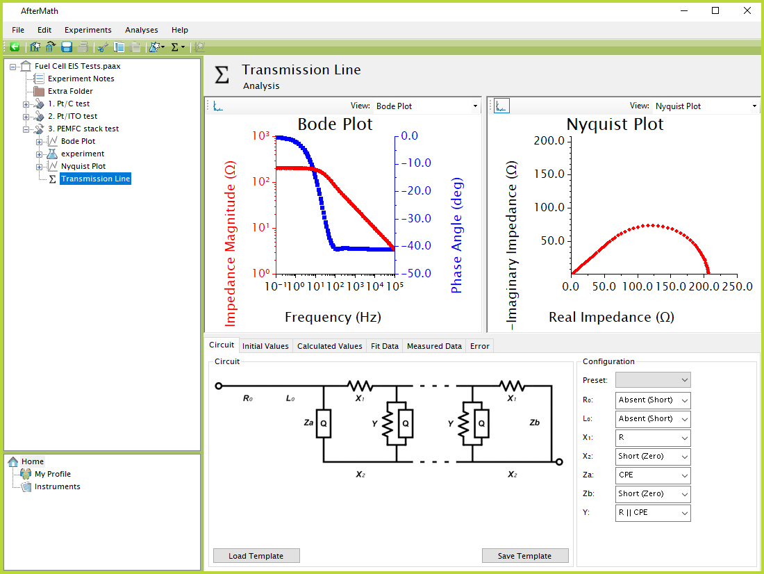
Figure 8. AfterMath Example Transmission Line Analysis
The third analysis type is called "Kramers-Kronig". The Kramers-Kronig analysis is a type of EIS diagnostic that appears similar to circuit fit, but unlike circuit fit it does not require any user input. Once the Kramers-Kronig option is selected, the test is automatically performed and the user is provided with corresponding error statistics and graphical results (see Figure 9). Once again, more information on Kramers-Kronig analysis can be found in other Pine Research Knowledgebase posts.
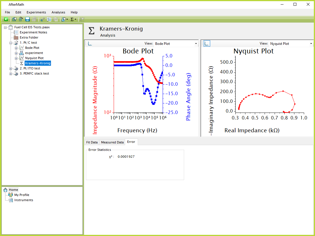
Figure 9. AfterMath Example Kramers-Kronig Analysis
The final analysis option is a simulation. A simulation is not restricted to EIS data and can be added underneath almost any node in an archive (see Figure 10). Similarly to a circuit fit, the first window that appears after adding a circuit simulation is the circuit library where a circuit model can be selected. Once the desired circuit model is chosen, the parameters can be adjusted as needed to observe their graphical effect on the Bode and Nyquist plots (see Figure 11). In a simulation, since there are no experimental data, there are no mathematical fitting operations that can be performed or statistical analyses to evaluate. However, the simulated circuit data can be easily copied and exported to another program if needed.
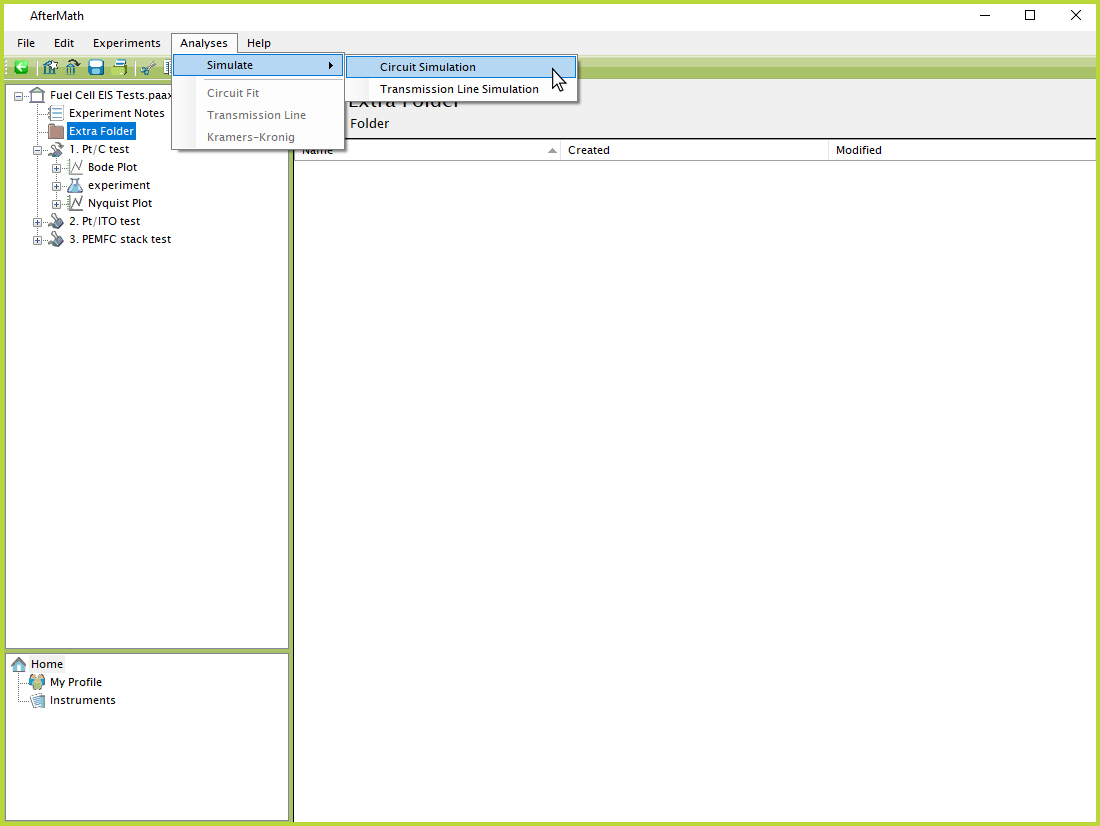
Figure 10. AfterMath Adding New Circuit Simulation
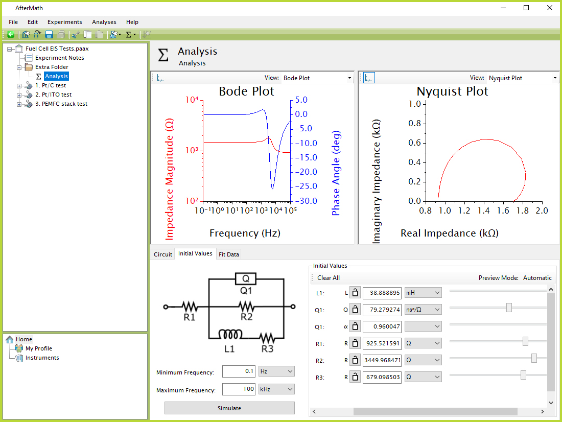
Figure 11. AfterMath Example Circuit Simulation