


Staircase Voltammetry (SCV)
Last Updated: 1/3/23 by Alex Peroff
1Technique Overview
Though there are similarities between SCV, Cyclic Voltammetry (CV),
 Cyclic Voltammetry (CV)
and Linear Sweep Voltammetry (LSV),
Linear Sweep Voltammetry (LSV)
SCV allows more control of the waveform that is applied to the working electrode. CV and LSV waveforms are optimized to take full advantage of the resolution of the potentiostat's digital-to-analog converter, while the waveform in SCV is designed for much higher sweep rates than typically encountered in CV or LSV.
Cyclic Voltammetry (CV)
and Linear Sweep Voltammetry (LSV),
Linear Sweep Voltammetry (LSV)
SCV allows more control of the waveform that is applied to the working electrode. CV and LSV waveforms are optimized to take full advantage of the resolution of the potentiostat's digital-to-analog converter, while the waveform in SCV is designed for much higher sweep rates than typically encountered in CV or LSV.
As with many other methods, users can initially sweep positively (towards an anodic limit) or negatively (toward a cathodic limit) initially. Below, typical NPV waveforms are shown for illustration, using only an increasing positive pulse sequence.
In the simplest case, when Segments (SN) = 1 (see Figure 1), potential steps, in time by period and in potential by amplitude, from an initial to final potential, sampling current at the specified width (time prior to next step) (see Figure 7).
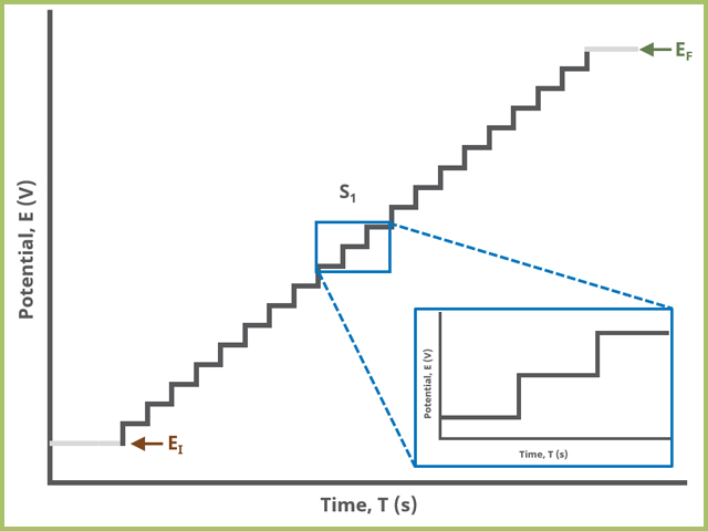
Figure 1. Staircase Voltammetry (SCV) One Segment Waveform
In the simplest case, when Segments (SN) = 2 (see Figure 2), potential steps, in time by period and in potential by amplitude, from an initial potential to vertex potential to final potential, sampling current at the specified width (time prior to next step) (see Figure 7).
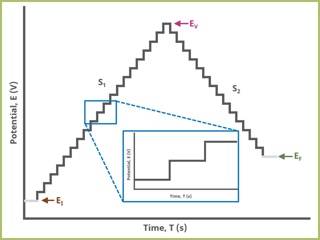
Figure 2. Staircase Voltammetry (SCV) Two Segment Waveform
When Segments (SN) = 3 (see Figure 3), potential steps, in time by period and in potential by amplitude, from an initial potential to vertex potential to upper potential to lower potential and to final potential, sampling current at the specified width (time prior to next step) (see Figure 7).
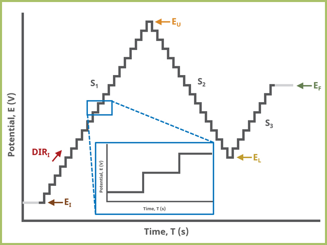
Figure 3. Staircase Voltammetry (SCV) Three Segment Waveform
2Fundamental Equations
One of the best ways to understand the fundamentals of SCV will be to compare it to the more common Cyclic Voltammetry (CV). Bard and Faulkner
 Bard, A. J.; Faulkner, L. A. Electrochemical Methods: Fundamentals and Applications, 2nd ed. Wiley-Interscience: New York, 2000.
provides a more exhaustive theoretical background and readers should consult this text for additional detail.
Bard, A. J.; Faulkner, L. A. Electrochemical Methods: Fundamentals and Applications, 2nd ed. Wiley-Interscience: New York, 2000.
provides a more exhaustive theoretical background and readers should consult this text for additional detail.
Unlike CV, where users specify a sweep rate (dE/dT,  ), the equivalent sweep rate in SCV is determined by the ratio of step amplitude and period (see Table 1 and Figure 7) as,
), the equivalent sweep rate in SCV is determined by the ratio of step amplitude and period (see Table 1 and Figure 7) as,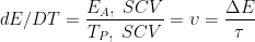
Under ideal conditions or conditions where uncompensated resistance is negligible, SCV should produce results identical to CV. At very high sweep rates, which is effectively possible with SCV as compared to CV, it is possible that kinetic effects can be masked as uncompensated resistance. A plot of  should extrapolate to
  when a large
  is caused only by uncompensated resistance.
should extrapolate to when a large is caused only by uncompensated resistance.Both CV and SCV utilize staircase waveforms (as opposed to truly linear waveforms generated in analog instruments); however, CV is optimized to take full advantage of the resolution of the potentiostat digital-to-analog converter (DAC). SCV gives you the ability to control the step height and duration enabling sweep rates greater than 10 V/s. Both methods provide some user control over current sampling. With CV, the parameter Alpha determines when the current is sampled,
Cyclic Voltammetry (CV)
where value of  means that the current is sampled immediately after the potential step whereas when
  means that the current is sampled immediately prior to the next potential step. In SCV, the parameter Sampling Control Width (defined in Table 1 and Figure 7, TW, SCV) determines the point (in time) along the potential step at which current is sampled before the next potential step; therefore, when TW, SCV = 5 ms and the Step period (defined in Table 1 and Figure 7, TS, SCV) = 10 ms in SCV, this corresponds to an Alpha of 50% in CV. Theoretically, it is ideal to sample at 1/4 of the sample window (
 in CV in the case of SCV,
means that the current is sampled immediately after the potential step whereas when means that the current is sampled immediately prior to the next potential step. In SCV, the parameter Sampling Control Width (defined in Table 1 and Figure 7, TW, SCV) determines the point (in time) along the potential step at which current is sampled before the next potential step; therefore, when TW, SCV = 5 ms and the Step period (defined in Table 1 and Figure 7, TS, SCV) = 10 ms in SCV, this corresponds to an Alpha of 50% in CV. Theoretically, it is ideal to sample at 1/4 of the sample window ( in CV in the case of SCV,
as described by Peixin He.
He, P. Conversion of Staircase Voltammetry to Linear Sweep Voltammetry by Analog Filtering. Anal. Chem., 1995, 67(5), 986-992.
The high-resolution DACs used in modern potentiostats make it unlikely that changing the point at which the current is sampled will noticeably alter the voltammogram of a species in solution. It is possible that changing the point at which current is sampled for a surface-bound species will introduce artifacts or alter the voltammogram significantly. Several have explored this point in the literature.
Hai, B. ; Tolmachev, Y. V. ; Loparo, K. A. ; Zanelli, C. ; Scherson, D. Cyclic versus Staircase Voltammetry in Electrocatalysis: Theoretical Aspects. J. Electrochem. Soc., 2010, 158(2), F15.
Stojek, Z. ; Osteryoung, J. Linear scan and staircase voltammetry of adsorbed species. Anal. Chem., 1991, 63(8), 839-841.
Christie, J. H. ; Osteryoung, R. A. Theoretical treatment of staircase voltammetric stripping from the thin film mercury electrode. Anal. Chem., 1976, 48(6), 869-872.
Bilewicz, R. ; Wikiel, K. ; Osteryoung, R. ; Osteryoung, J. General equivalence of linear scan and staircase voltammetry: experimental results. Anal. Chem., 1989, 61(9), 965-972.
Kalapathy, U. ; Tallman, D. E. Equivalence of staircase and linear sweep voltammetries for reversible systems including conditions of convergent diffusion. Anal. Chem., 1992, 64(22), 2693-2700.
3Experimental Setup in AfterMath
To perform a staircase voltammetry experiment in AfterMath, choose Staircase Voltammetry (SCV) from the Experiments menu (see Figure 4).
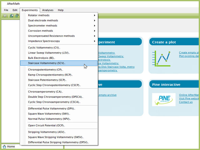
Figure 4. Staircase Voltammetry (SCV) Experiment Menu Selection in AfterMath
Doing so creates an entry within the archive, called SCV Parameters. In the right pane of the AfterMath application, several tabs will be shown (see Figure 5).
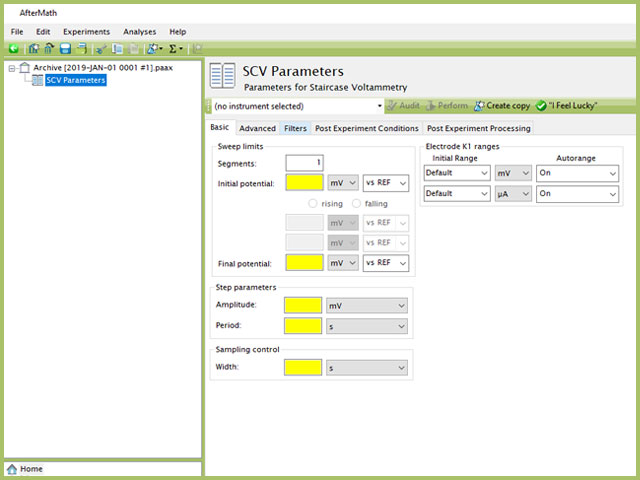
Figure 5. Staircase Voltammetry (SCV) Experiment Basic Tab
The experiment sequence is
Induction Period → Staircase → Relaxation Period → Post-Experiment Idle Conditions
Continue reading for detailed information about the fields on each unique tab.
3.1Basic Tab
The basic tab contains fields for the fundamental parameters necessary to perform an SCV experiment. AfterMath shades fields with yellow when a required entry is blank and shades fields pink when the entry is invalid (see Figure 6).
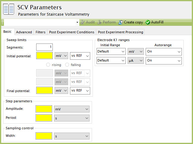
Figure 6. Staircase Voltammetry (SCV) Basic tab in AfterMath
During the induction period,
Induction Period
a set of initial conditions are applied to the electrochemical cell and the cell equilibrates at these conditions. Data are not collected during the induction period, nor are they shown on the plot during this period. Users will define induction period parameters on the Advanced Tab.
After the induction period, the potential of the working electrode is stepped through a series of increasing steps from the Initial potential to the Final potential at a specified period (TP, SCV). The potential is incremented with each successive pulse according to the Pulse amplitude (EA, SCV). Current is measured at the time defined by Pulse width (TW, SCV), which is the time before the next step. In a typical experiment, Segments = 1 and there is a single series of increasing steps. Some may want to reverse the pulses (move in the opposite direction), accomplished by adjusting the number of segments to be > 1. Refer to Figures 1, 2, and 3 for examples of such SCV waveforms that vary based on the number of segments.
The parameter settings for step-type experiments are often not as clear as with something more simple like Cyclic Voltammetry (a sweep method ). Refer to Figure 2 above when understanding each parameter of the NPV pulse. Further, clicking "AutoFill" ("I Feel Lucky" in older versions of AfterMath) provides reasonable starting parameters if you are unsure of typical values used in these experiments. Most often, research journal articles describe the NPV pulse sequence used, which can be replicated using AfterMath.
The experiment concludes with a relaxation period.
Relaxation Period
During the relaxation period, a set of final conditions (specified on the Advanced tab) are applied to the electrochemical cell and the cell equilibrates at these conditions (set on the Advanced Tab). Data are not collected during the induction period, nor are they shown on the plot during this period.
At the end of the relaxation period, the post-experiment idle conditions are applied to the cell and the instrument returns to the idle state.
A plot of the typical experiment sequence, containing labels of the fields on the Basic tab, helps to illustrate the sequence of events in an NPV experiment (see Table 1 and Figure 7).
| Group Name | Field Name | Symbol |
| Sweep (Sweep limits) | Segments |  |
| Sweep (Sweep limits) | Initial Potential |  |
| Sweep (Sweep limits) | Initial Direction |  |
| Sweep (Sweep limits) | Upper Potential |  |
| Sweep (Sweep limits) | Vertex Potential |  |
| Sweep (Sweep limits) | Lower Potential |  |
| Sweep (Sweep limits) | Final Potential |  |
| Normal Pulse (Pulse parameters) |
Baseline |  |
| Normal Pulse (Pulse parameters) |
Width |  |
| Normal Pulse (Pulse parameters) |
Period |  |
| Normal Pulse (Pulse parameters) |
Increment |  |
| Normal Pulse (Pulse parameters) |
Sampling Width |  |
Table 1. Basic Tab Group Names, Field Names, and Symbols.
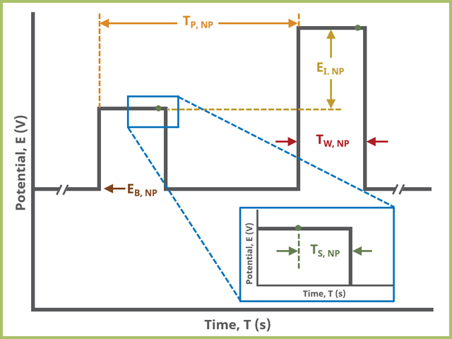
Figure 7. Normal Pulse Voltammetry (NPV) Pulse Parameter Field Diagram
3.2Advanced Tab
3.3Ranges, Filters, and Post Experiment Conditions Tab
4Typical Result
Typical results for a 1.5 mM solution of Ferrocene in 0.1 M Bu4NClO4/MeCN are shown below. Two different sweep rates have been shown along with different Sample windows.
5Example Applications
The first example uses staircase voltammetry to generate sweep rates as high as 200 V/s. Baur et al.
Baur, J. E.; Kristensen, E. W.; May, L. J.; Wiedemann, D. J.; Wightman, R. M. Fast-scan voltammetry of biogenic amines. Anal. Chem., 1988, 60(13), 1268-1272.
used staircase voltammetry to detect biogenic amines. These high sweep rates have three advantages:
- High sweep rates allow for the detection of these species while preventing the formation of an insulating layer.
- High sweep rates allow extracellular detection of these amines in the brain
- High sweep rates discriminate against chemical events after the initial electron transfer.
In another example, Heering et al.
Heering, H. A.; Mondal, M. S.; Armstrong, F. A. Using the Pulsed Nature of Staircase Cyclic Voltammetry To Determine Interfacial Electron-Transfer Rates of Adsorbed Species. Anal. Chem., 1999, 71(1), 174-182.
used SCV to measure electron transfer rates of an adsorbed species. The researchers showed that SCV becomes independent of step amplitude and similar to CV at high sweep rates ( ) if the current is sampled at 1/2 of the step period. The researchers determined the rate constant (ko) and n for adsorbed yeast cytochrome c peroxidase. Values obtained from SCV were comparable to more traditional methods such as chronoamperometry (CA).
Chronoamperometry (CA)
) if the current is sampled at 1/2 of the step period. The researchers determined the rate constant (ko) and n for adsorbed yeast cytochrome c peroxidase. Values obtained from SCV were comparable to more traditional methods such as chronoamperometry (CA).
Chronoamperometry (CA)
) if the current is sampled at 1/2 of the step period. The researchers determined the rate constant (ko) and n for adsorbed yeast cytochrome c peroxidase. Values obtained from SCV were comparable to more traditional methods such as chronoamperometry (CA).
6References
- Bard, A. J.; Faulkner, L. A. Electrochemical Methods: Fundamentals and Applications, 2nd ed. Wiley-Interscience: New York, 2000.
- He, P. Conversion of Staircase Voltammetry to Linear Sweep Voltammetry by Analog Filtering. Anal. Chem., 1995, 67(5), 986-992.
- Hai, B. ; Tolmachev, Y. V. ; Loparo, K. A. ; Zanelli, C. ; Scherson, D. Cyclic versus Staircase Voltammetry in Electrocatalysis: Theoretical Aspects. J. Electrochem. Soc., 2010, 158(2), F15.
- Stojek, Z. ; Osteryoung, J. Linear scan and staircase voltammetry of adsorbed species. Anal. Chem., 1991, 63(8), 839-841.
- Christie, J. H. ; Osteryoung, R. A. Theoretical treatment of staircase voltammetric stripping from the thin film mercury electrode. Anal. Chem., 1976, 48(6), 869-872.
- Bilewicz, R. ; Wikiel, K. ; Osteryoung, R. ; Osteryoung, J. General equivalence of linear scan and staircase voltammetry: experimental results. Anal. Chem., 1989, 61(9), 965-972.
- Kalapathy, U. ; Tallman, D. E. Equivalence of staircase and linear sweep voltammetries for reversible systems including conditions of convergent diffusion. Anal. Chem., 1992, 64(22), 2693-2700.
- Baur, J. E.; Kristensen, E. W.; May, L. J.; Wiedemann, D. J.; Wightman, R. M. Fast-scan voltammetry of biogenic amines. Anal. Chem., 1988, 60(13), 1268-1272.
- Heering, H. A.; Mondal, M. S.; Armstrong, F. A. Using the Pulsed Nature of Staircase Cyclic Voltammetry To Determine Interfacial Electron-Transfer Rates of Adsorbed Species. Anal. Chem., 1999, 71(1), 174-182.