Normal Pulse Voltammetry (NPV)

Last Updated: 1/5/23 by Alex Peroff

Capable Potentiostats

AFTERMATH LINKS

Article Contents/Section Navigation

1Technique Overview

Normal Pulse Voltammetry (NPV) is a potentiostatic method that offers some advantages to common techniques like Cyclic Voltammetry (CV), in that the waveform is a series of pulses that are increasing in potential amplitude. The way in which the current is measured at each pulse aids in minimizing the measurement of background (charging) current. Related pulse-type methods include Differential Pulse Voltammetry (DPV) and Square Wave Voltammetry (SWV).

Normal Pulse Voltammetry (NPV) is a derivative technique of Normal Pulse Polarography (NPP). NPP is a technique that was traditionally used with Dropping Mercury Electrodes and Static Mercury Dropping Electrodes. The waveform for the two techniques is the same; however, it is appropriate to use the term “Normal Pulse Voltammetry” when referring to the application of the waveform to nonpolarographic electrodes.

As with many other methods, users can initially sweep positively (towards an anodic limit) or negatively (toward a cathodic limit) initially. Below, typical NPV waveforms are shown for illustration, using only an increasing positive pulse sequence.

INFO: Initial sweep direction can be positive-increasing or negative increasing. Not all possibilities have been provided as examples in this article. Users must tailor their parameters to suit their specific electrochemistry. Contact us with any questions or additional assistance.

In the simplest case, when Segments (S_N) = 1 (see Figure 1), increasing potential pulses step from a common baseline in a linear fashion, from an initial to final potential, sampling current at specified intervals (see Figure 7).

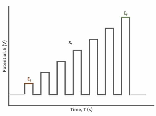
Figure 1. Normal Pulse Voltammetry (NPV) One Segment Waveform

Current sampling occurs at the same time in each pulse of the NPV waveform. For each pulse, the current is sampled as a function of the pulse sequence, $i_{sample}(T^*)$ , which is determined as

$T^*=T_{W,\;NP}-T_{S,\;NP}$

where $T_{W,\:NP}$ is the pulse width and $T_{S,\:NP}$ is the sampling width (see Table 1 and Figure 7).

When Segments (S_N) = 2 (see Figure 2), increasing potential pulses step from a common baseline in a linear fashion, from an initial potential to vertex potential, at which time the NPV pulses decrease until reaching the final potential. Again, the current is sampled in the same fashion as NPV experiments with other Segment values.

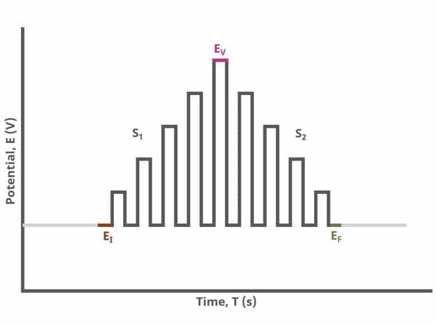
Figure 2. Normal Pulse Voltammetry (NPV) Two Segment Waveform

When Segments (S_N) = 3 (see Figure 3), increasing potential pulses step from a common baseline in a linear fashion, from an initial potential to upper potential, then from upper potential to lower potential, and finally from lower potential to final potential. Throughout each segment, the NPV pulses increases/decreases until reaching the next significant potential value supplied to AfterMath. Again, the current is sampled in the same fashion as NPV experiments with other Segment values (see Figure 7).

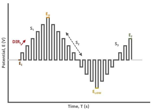
Figure 3. Normal Pulse Voltammetry (NPV) Three Segment Waveform

2Fundamental Equations

Consider the reaction

$O + ne^- \rightleftharpoons R$

where $O$ is reduced in a one-electron reaction to $R$ with formal potential $E^0$ . The application of a baseline potential should be sufficiently positive of $E^0$ such that no faradaic current flows. After a period of time $({\tau}')$ , typically 100 - 5000 ms, the potential of the working electrode is stepped to a more negative value for a period of time. The total time from the application of the baseline potential through the application of the potential pulse is ${\tau}$ .

The potential pulse is incrementally increased with each cycle. As the potential of the working electrode approaches $E^0$ faradaic current flows due to the reduction of $O$ to $R$ . Upon the application of the baseline potential in the next cycle, $R$ is oxidized back to $O$ . When the potential of the working electrode gets sufficiently negative of $E^0$ , $O$ is reduced to $R$ at a maximum rate and the current levels off to a plateau The magnitude of this current plateau is given by

$\displaystyle i_{d,NPV} = \frac{nFAD_O^{1/2}C_O^*}{{\pi}^{1/2}({\tau}-{\tau}')^{1/2}}$

where $n$ is the number of electrons, $F$ is Faraday's Constant ( $96,485 \; C/mol$ ), $A$ is the electrode area ( $cm^2$ ), $D$ is the diffusion coefficient( $cm^2/s$ ), $C$ is the concentration ( $mol/cm^3$ ) and ${\tau}'$ and ${\tau}$ are as described above.

As seen in the Sample Experiments section, RNPV gives the same wave shape but not the same current. These results are analogous to DPSCA where the current during the forward pulse is different than the current in the reverse pulse. Here in RNPV, the baseline potential is such that $O$ is being reduced to $R$ at a maximum rate. As the potential of the working electrode approaches $E^0$ a faradaic current flows due to the oxidation of $R$ to $O$ . Once the potential of the working electrode is sufficiently positive of $E^0$ , $R$ is being oxidized at a maximum rate and the current plateaus. The magnitude of this current plateau is given by

$\displaystyle i_{d,RPV} = \frac{nFAD_O^{1/2}C_O^*}{{\pi}^{1/2}}\left[{\frac{1}{({\tau}-{\tau}')^{1/2}}}-{\frac{1}{{\tau}^{1/2}}}\right]$

where the parameters are as described above. Notice that in the Sample Experiments section, there is a slight anodic current flowing at the beginning of the experiment. The magnitude of this current is given by the equation

$\displaystyle i_{d,DC} = \frac{nFAD_O^{1/2}C_O^*}{{\pi}^{1/2}{\tau}^{1/2}}$

where the parameters are as described above. The magnitude of this current is the difference between the NPV and RNPV currents.

Bard and Faulkner provide a summary and description of normal pulse voltammetry as do Kissinger and Heinemann.

3Experimental Setup in AfterMath

To perform a normal pulse voltammetry experiment in AfterMath, choose Normal Pulse Voltammetry (NPV) from the Experiments menu (see Figure 4).

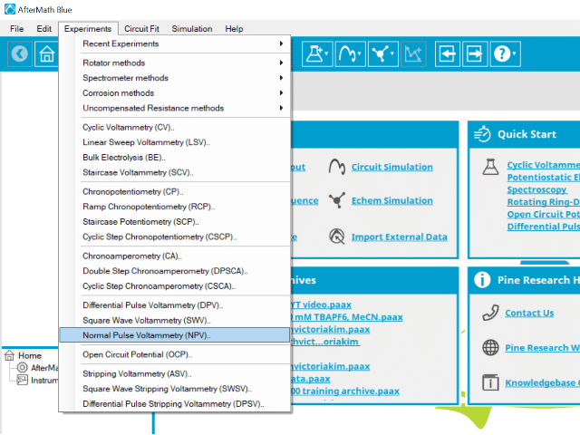
Figure 4. Normal Pulse Voltammetry (NPV) Experiment Menu Selection in AfterMath

Doing so creates an entry within the archive, called NPV Parameters. In the right pane of the AfterMath application, several tabs will be shown (see Figure 5).

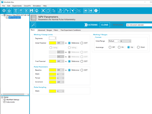
Figure 5. Normal Pulse Voltammetry (NPV) Experiment Parameters

As with most Aftermath methods, the experiment sequence is

Induction Period → Pulse Sequence → Relaxation Period → Post-Experiment Idle Conditions

Continue reading for detailed information about the fields on each unique tab.

3.1Basic Tab

TIP: Click the AutoFill button ("I Feel Lucky" prior to May 2019) on the top bar in AfterMath to automatically fill all required parameters with reasonable starting values. While the values provided may not be appropriate for your specific system, they are reasonable parameters with which to start your experiment, especially if you are new to the method.

The basic tab contains fields for the fundamental parameters necessary to perform an NPV experiment. AfterMath shades fields with yellow when a required entry is blank and shades fields pink when the entry is invalid (see Figure 6).

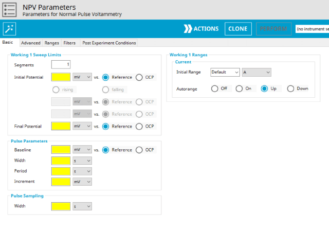
Figure 6. Normal Pulse Voltammetry (NPV) Basic tab in AfterMath

During the induction period, a set of initial conditions are applied to the electrochemical cell and the cell equilibrates at these conditions. Data are not collected during the induction period, nor are they shown on the plot during this period. Users will define induction period parameters on the Advanced Tab.

After the induction period, the potential of the working electrode is stepped through a series of increasing pulses from the Initial potential to the Final potential. The potential is incremented with each successive pulse according to the Pulse increment. Current is measured at the time obtained by subtracting the Pulse sampling width window from the Pulse width. In a typical experiment, Segments = 1 and there is a single series of increasing pulses. Some may want to reverse the pulses (move in the opposite direction), accomplished by adjusting the number of segments to be > 1. By adjusting the number of segments, users can create variants of the NPV technique. Cyclic Normal Pulse Voltammetry consists of cycling (through a series of potential pulses also) the potential of the working electrode between an Upper potential and a Lower potential (Segments = 2 or 3). Reverse Normal Pulse Voltammetry is a variant of NPV where you choose to apply a Baseline potential in a region where the Faradaic current is flowing at a maximal rate ( $>200 \; mV$ from $E^0$ ). Refer to Figures 1, 2, and 3 for examples of such NPV waveforms that vary based on number of segments.

The parameter settings for pulse-type experiments are often not as clear as with something more simple like Cyclic Voltammetry (a sweep method ). Refer to Figure 2 above when understanding each parameter of the NPV pulse. Further, clicking "AutoFill" ("I Feel Lucky" in older versions of AfterMath) provides reasonable starting parameters if you are unsure of typical values used in these experiments. Most often, research journal articles describe the NPV pulse sequence used, which can be replicated using AfterMath.

The experiment concludes with a relaxation period. During the relaxation period, a set of final conditions (specified on the Advanced tab) are applied to the electrochemical cell and the cell equilibrates at these conditions (set on the Advanced Tab). Data are not collected during the induction period, nor are they shown on the plot during this period.

At the end of the relaxation period, the post-experiment idle conditions are applied to the cell and the instrument returns to the idle state.

A plot of the typical experiment sequence, containing labels of the fields on the Basic tab, helps to illustrate the sequence of events in an NPV experiment (see Table 1 and Figure 7).

The table below lists the group and field names and symbols for each parameter associated with this experiment (see Table 1).

Group Name	Field Name	Symbol
Sweep (Sweep limits)	Segments	$S_N$
Sweep (Sweep limits)	Initial Potential	$E_I$
Sweep (Sweep limits)	Initial Direction	$DIR_I$
Sweep (Sweep limits)	Upper Potential	$E_U$
Sweep (Sweep limits)	Vertex Potential	$E_V$
Sweep (Sweep limits)	Lower Potential	$E_{LOW}$
Sweep (Sweep limits)	Final Potential	$E_F$
Normal Pulse (Pulse parameters)	Baseline	$E_{B, \;NP}$
Normal Pulse (Pulse parameters)	Width	$T_{W, \;NP}$
Normal Pulse (Pulse parameters)	Period	$T_{P, \;NP}$
Normal Pulse (Pulse parameters)	Increment	$E_{I, \;NP}$
Normal Pulse (Pulse parameters)	Sampling Width	$T_{S, \;NP}$

Table 1. Basic Tab Group Names, Field Names, and Symbols.

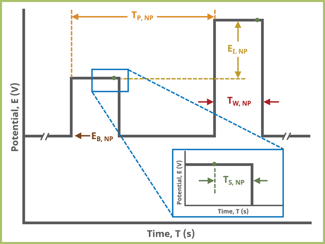
Figure 7. Normal Pulse Voltammetry (NPV) Pulse Parameter Field Diagram

3.2Advanced Tab

The NPV Advanced tab contains groups for Induction Period, Relaxation Period, and iR Compensation (see Figure 8).

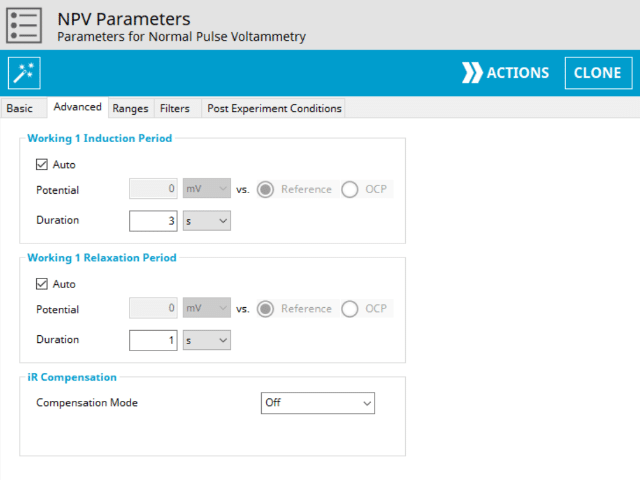
Figure 8. Normal Pulse Voltammetry (NPV) Experiment Advanced Tab in AfterMath

Induction Period is the first step in an NPV experiment if the Duration is >0 s. During the induction period, the specified current is applied to the cell for the specified duration. During this period, data are not collected. The Induction Period is believed to "calm" the cell prior to intentional perturbation. More on Induction Period is found within the knowledgebase.

Relaxation Period is the last step in an NPV experiment if the Duration is >0 s. During the relaxation period, the specified current is applied to the cell for the specified duration. During this period, data are not collected. The Relaxation Period is believed to "calm" the cell after intentional perturbation. More on Relaxation Period is found within the knowledgebase.

Lastly, the iR Compensation group allows users to adjust the cell feedback to accommodate a known resistive drop between working and reference electrodes. Not all potentiostats from Pine Research support iR compensation. The WaveDriver series support iR compensation by positive feedback and current interrupt. The WaveDriver 100, WaveDriver 200, and WaveDriver 40 support EIS-based iR compensation. The WaveNow series (including the WaveNano and WaveNow^XV WaveNowXV Potentiostat/Galvanostat Basic Bundle ) and the CBP bipotentiostat do not support iR compensation of any type. More information about iR compensation, including understanding how it works and how to determine the resistance, consult the knowledgebase article on the topic.

The general experimental flow for an NPV experiment is provided below (see Figure 9), highlighting the Induction period, NPV Pulse Sequence, and Relaxation period. Following the relaxation period, the post-experiment conditions are applied.

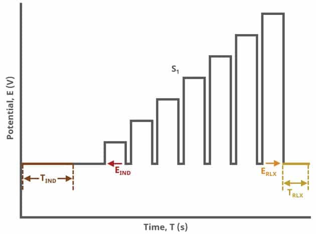
Figure 9. Normal Pulse Voltammetry (NPV) General Experiment Sequence in AfterMath

3.3Ranges, Filters, and Post Experiment Conditions Tab

In nearly all cases, the groups of fields on the Ranges tab are already present on the Basic tab. The Ranges tab shows an Electrode Range group and depending on the experiment shows either, or both, current and potential ranges and the ability to select an autorange function. The fields on this tab are linked to the same fields on the Basic tab (for most experiments). Changing the values on either the Ranges tab or on the Basic tab changes the other set. In other words, the values selected for these fields will always be the same on the Ranges tab and on the Basic tab. More on ranges is found within the knowledgebase, as is for autorange.

The Filters tab provides access to potentiostat hardware filters, including stability, excitation, current response, and potential response filters. Pine Research recommends that users contact us for help in making changes to hardware filters. Advanced users may have an easier time changing the automatic settings on this tab. Filter settings fields are shown for WK1 (working electrode #1) as well as for WK2 (working electrode #2) regardless of the potentiostat connected to AfterMath.

By default, the potentiostat disconnects from the electrochemical cell at the end of an experiment. There are other options available for what these post-experiment conditions can be and are controlled by setting options on the Post Experiment Conditions tab.

4Sample Experiment

The typical results for NPV of a $0.5 \; mM$ solution of Ferrocene in $0.1 \; M \; Bu_4NClO_4/MeCN$ show a sigmoid-shaped curve (see Figure 10). In this experiment, the specific parameters were as follows:

2 mm OD Pt WE
Pt mesh CE
Baseline Potential = 0.1 V
Initial Potential = 0.25 V
Final Potential = 1 V
Pulse increment = 10 mV
Pulse period = 100 ms
Pulse width = 10 ms
Sample width = 1 ms

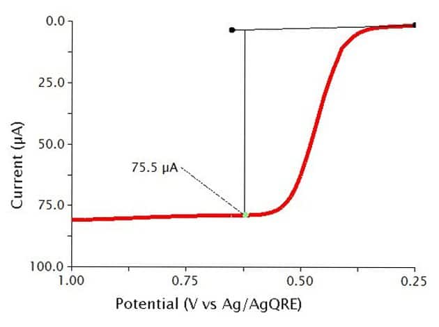
Typical Normal Pulse Voltammetry (NPV) Experimental Data

Figure 10. Typical NPV results for 0.5 mM Ferrocene in 0.1 Bu₄NClO₄/MeCN

The typical results for Reverse Normal Pulse Voltammetry (RNPV) of a 0.5 mM solution of Ferrocene in $0.1 \; M \; Bu_4NClO_4/MeCN$ show a sigmoid-shaped curve (see Figure 11). In this experiment, the specific parameters were as follows:

2 mm OD Pt WE
Pt mesh CE
Baseline Potential = 1 V
Initial Potential = 0.75 V
Final Potential = 0 V
Pulse increment = 10 mV
Pulse period = 100 ms
Pulse width = 10 ms
Sample width = 1 ms

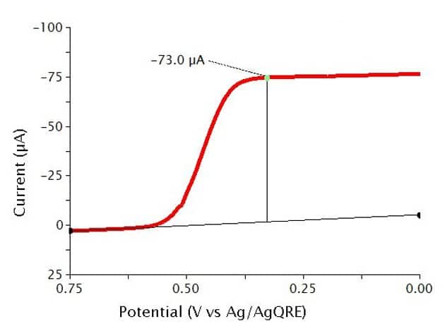
Typical Reverse Normal Pulse Voltammetry (RNPV) Experimental Data

Figure 11. Typical RNPV results for 0.5 mM Ferrocene in 0.1 Bu₄NClO₄/MeCN

The typical results for Cyclic Normal Pulse Voltammetry (CNPV) of a 0.5 mM solution of Ferrocene in $0.1 \; M \; Bu_4NClO_4/MeCN$ show two sigmoid-shaped curves (see Figure 12, same conditions as for those used in generating the data in Figure 11). Since Ferrocene is fully-reversible electrochemically, the two sigmoids overlap.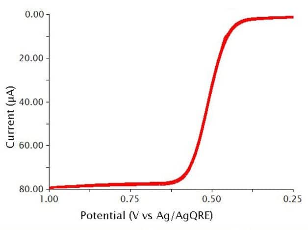

Typical Cyclic Pulse Voltammetry (CNPV) Experimental Data

Figure 12. Typical CNPV results for 0.5 mM Ferrocene in 0.1 Bu₄NClO₄/MeCN

5Example Applications

The first example uses NPV to confirm a diffusion coefficient calculated initially by chronoamperometry (CA). Oyaizu et al. produced an organic radical polymer to be used in charge-storage applications. The current in this case is controlled by diffusion of the counter ion through the film.

In another example, Welch et al. use NPV to measure a diffusion coefficient. They measured the diffusion coefficients of a free and DNA-bound organo-metallic complex. NPV was superior to CV in this instance due to the low concentration of species in solution.

In this third example, Osteryoung et al. use Reverse Normal Pulse Voltammetry (RNPV). The usefulness of RNPV lies in its ability to examine products from chemical reactions that take place after an electrochemical reaction. Osteryoung et al. used RNPV to obtain the backwards rate constant and equilibrium constant for the dimerization of N-methyl-2-carbomethoxypyridinium radical, produced after the electrochemical reduction of the N-methyl-2-carbomethoxypyridinium ion.

How can we help? What do you want to learn? Search our knowledgebase.

Voltammetric Methods

Normal Pulse Voltammetry (NPV)

ARTICLE TAGS

Capable Potentiostats

RELATED PAGES

AFTERMATH LINKS

Article Contents/Section Navigation

1Technique Overview

2Fundamental Equations

3Experimental Setup in AfterMath

3.1Basic Tab

3.2Advanced Tab

3.3Ranges, Filters, and Post Experiment Conditions Tab

4Sample Experiment

5Example Applications

6References

Questions? Find Answers.

Software

Applications

Theory

Product Specifications