1Technique Overview
Double Step Chronoamperometry (DPSCA) is a potential step method and is also known as double constant potential bulk electrolysis, double controlled potential amperometry, and double potential pulse electrolysis. In its most simple case, DPSCA is the measurement of current vs. time due to a change (step, pulse) in potential, followed by a reverse change (step, pulse).
Double Step Chronoamperometry (DPSCA) is a widely used method in electrochemistry, due in part to its relative ease of implementation and analysis. DPSCA is highly sensitive, as most electrochemical methods are; however, DPSCA is poorly selective. In an unstirred cell, in response to a potential step perturbation, electrochemically active species will diffuse to the surface of the working electrode as a function of the potential applied. At the onset of a forward potential step, a large current arising from ion flux to the electrode surface to balance the change in potential gives rise to a capacitive current, which decays rapidly (just like any RC circuit
). The concentration of electrochemically active species near the electrode surface decays with distance from the electrode and the arrival of species to the surface is diffusion limited; therefore, Faradaic current near the electrode surface decays over time as the mass transport limit is reached. The same process, but opposite reaction, arises in the reverse step. These currents provide a typical exponential decay curve, which is described by the Cottrell equation.
DPSCA is a technique that is often used to elucidate mechanisms related to coupled homogeneous reactions preceding or following an electrode reaction. The simplest coupled homogeneous reactions are Electrochemical-Chemical (EC) and Chemical-Electrochemical (CE) reactions. Bard and Faulkner give a more detailed description of using DPSCA to elucidate mechanisms.
2Fundamental Equations
The following is a basic description of the theory behind DPSCA. Please see the literature for a more detailed description of the technique.
Consider the general reaction
with a formal potential

. In general, the potential step applied to the working electrode should be sufficiently more negative than
such that reduction of

to

is complete at the surface of the electrode (
i.e., surface concentration of
at the electrode surface is

). When this occurs, the current is diffusion-limited, much like the current that flows in cyclic voltammetry
after the potential of the electrode sweeps past

.
When the current is diffusion-limited in CA, as stated in the description of chronamperometry,
the time-dependent current transient in a diffusion-limited chronoamperometry experiment is governed by the Cottrell equation
where

is current,

is the number of electrons transferred in the half reaction,

is Faraday's Constant (96,485 C/mol)
,

is the area of the electrode,

is the diffusion coefficient,

is the initial concentration, and

is time. In DPSCA, the time of the transition must be considered. The current transient for the second step, provided it produces diffusion-limited current, is governed by the equation first described by Kambara
where

is the transition time and the other parameters are as above.
3Experimental Setup in AfterMath
To perform a double step chronoamperometry experiment in AfterMath, choose Double Step Chronoamperometry (DPSCA) from the Experiments menu (see Figure 1).
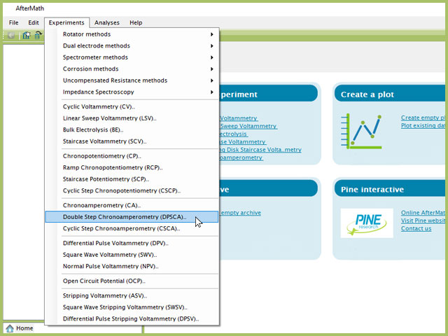
Figure 1. Double Step Chronoamperometry (DPSCA) Experiment Menu Selection in AfterMath
Doing so creates an entry within the archive, called DPSCA Parameters. In the right pane of the AfterMath application, several tabs will be shown (see Figure 2).
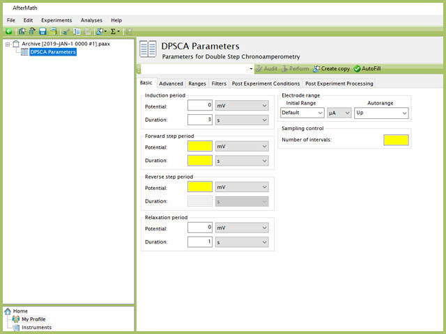
Figure 2. Double Potential Step Chronopotentiometry (DPSCA) Experiment Basic Tab in AfterMath
As with most Aftermath methods, the experiment sequence is
Induction Period → Electrolysis Period (Step 1 → 2) → Relaxation Period → Post-Experiment Idle Conditions
Like many experiments, the Induction and Relaxation Periods are on the Advanced Tab. The parameters for a DPSCA experiment are fairly simple compared to other methods in AfterMath.
In general, enter minimum required parameters on the Basic tab and press "Perform" to run an experiment. AfterMath will perform a quick audit of the parameters you entered to ensure their validity and appropriateness for the chosen instrument, followed by the initiation of the experiment. In some cases, users may desire to adjust additional settings such as filters, post-experiment conditions, and post-experiment processing before clicking the "Perform" button. Continue reading for detailed information about the fields on each unique tab.
3.1Basic Tab
TIP: Click the AutoFill button ("I Feel Lucky" prior to May 2019) on the top bar in AfterMath to automatically fill all required parameters with reasonable starting values. While the values provided may not be appropriate for your specific system, they are reasonable parameters with which to start your experiment, especially if you are new to the method.
The basic tab contains fields for the fundamental parameters necessary to perform a DPSCA experiment. AfterMath shades fields with yellow when a required entry is blank and shades fields pink when the entry is invalid (see Figure 3).
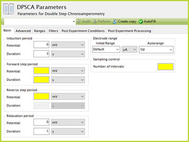
Figure 3. Double Potential Step Chronoamperometry (DPSCA) Experiment Basic Tab in AfterMath
During the induction period,
a set of initial conditions are applied to the electrochemical cell and the cell equilibrates at these conditions. Data are not collected during the induction period, nor are they shown on the plot during this period.
After the induction period, the potential applied to the working electrode is stepped to the specified value for the duration of the experiment, which is called the Forward step period. The potentiostatic circuit of the instrument maintains constant applied potential relative to the reference electrode while simultaneously measuring the current at the working electrode. During the electrolysis period, potential and current at the working electrode are recorded at regular intervals as specified on the Basic tab for the first (forward) potential step and then the second (reverse) potential step in the sequence. There is no pause between the two steps and potential is nearly instantaneously stepped from the first to second electrolysis potential.
Sampling control defines the number of intervals (number of data points) collected during the electrolysis period. With Electrolysis period duration, a sampling rate can be defined as,
Users should enter a number of intervals that their analysis requires. Commonly, DPSCA experiments are sampled at a lower rate (1 sample/s). Not all sampling rates are allowed due to differences in hardware (WaveNow series vs. WaveDriver series, for example).
NOTE: Not all sampling rates are possible. When users enter a number of intervals that is not allowed, AfterMath will prompt the user with an "Interval too short" error. Change the number of intervals and try again. In general, integer values at moderate rates are most often possible.
The Electrode Range group contains the initial current field.
These field settings within the Electrode Range group explicitly define the initial current range used by the potentiostat during the experiment. Additionally, a field for Autorange control for both potential and current appear on this tab. Autorange employs algorithms to adjust the current and potential ranges, as needed, to the most appropriate ranges available to match the measured signal(s). More information on autorange is available elsewhere on the knowledgebase.
The experiment concludes with a relaxation period.
During the relaxation period, a set of final conditions (specified on the Advanced tab) are applied to the electrochemical cell and the cell equilibrates at these conditions. Data are not collected during the induction period, nor are they shown on the plot during this period.
A plot of the typical experiment sequence, containing labels of the fields on the Basic tab, helps to illustrate the sequence of events in a DPSCA experiment (see Table 1 and Figure 4).
The table below lists the group and field names and symbol for each parameter associated with this experiment (see Table 1).
| Group Name |
Field Name |
Symbol |
| Induction Period |
Potential |
 |
| Induction Period |
Duration |
 |
Electrolysis Period (Step 1)
(Forward Step Period) |
Potential |
 |
Electrolysis Period (Step 1)
(Forward Step Period) |
Duration |
 |
Electrolysis Period (Step 2)
(Reverse Step Period) |
Potential |
 |
Electrolysis Period (Step 2)
(Reverse Step Period) |
Duration |
 |
| Relaxation Period |
Potential |
 |
| Relaxation Period |
Duration |
 |
| Sampling Control |
Number of Intervals |
 |
Table 1. Basic Tab Group Names, Field Names, and Symbols.
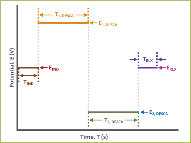
Figure 4. Double Potential Step Chronoamperometry (DPSCA) Basic Tab Field Diagram
At the end of the relaxation period, the post-experiment idle conditions
are applied to the cell, the post-experiment processing tasks perform, and the instrument returns to the idle state. The default plot generated from the data is current vs. time.
3.2Advanced Tab
The DPSCA Advanced tab contains two groups for iR Compensation and for Experiment End Trigger (see Figure 5).
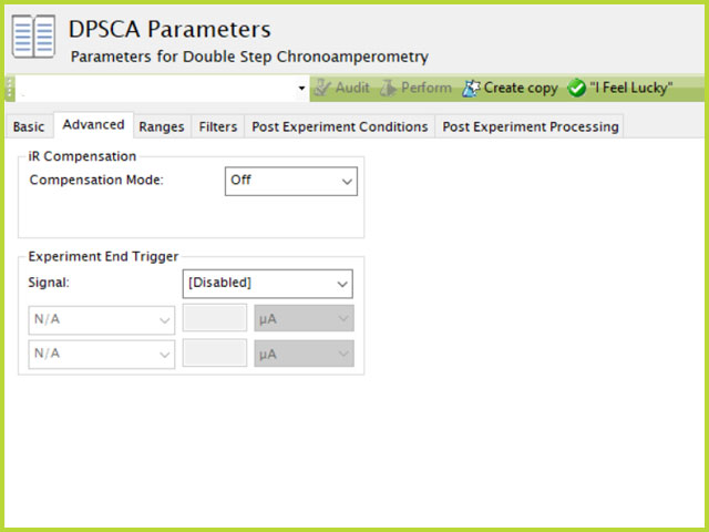
Figure 5. Double Potential Step Chronoamperometry (DPSCA) Experiment Advanced Tab in AfterMath
Detailed description of the iR Compensation Mode is provided elsewhere on the knowledgebase.
This mode is used to correct for uncompensated resistance in the electrochemical cell.
In a DPSCA experiment, the researcher may want to have AfterMath monitor the response and then stop the experiment at a specific current, potential, and/or charge. This value is called a trigger and is set in the Experiment End Trigger group on the Advanced tab (see Figure 5). For DPSCA, the signals for the trigger can be potential, current, or charge. Details on the End Trigger settings are found elsewhere in the knowledgebase.
3.3Ranges, Filters, and Post Experiment Conditions Tab
In nearly all cases, the groups of fields on the Ranges tab are already present on the Basic tab. The Ranges tab shows an Electrode Range group and depending on the experiment shows either, or both, current and potential ranges and the ability to select an autorange function. The fields on this tab are linked to the same fields on the Basic tab (for most experiments). Changing the values on either the Ranges tab or on the Basic tab changes the other set. In other words, the values selected for these fields will always be the same on the Ranges tab and on the Basic tab. More on ranges is found within the knowledgebase,
as is for autorange.
The Filters tab provides access to potentiostat hardware filters, including stability, excitation, current response, and potential response filters. Pine Research recommends that users contact us
for help in making changes to hardware filters. Advanced users may have an easier time changing the automatic settings on this tab. Filter settings fields are shown for WK1 (working electrode #1) as well as for WK2 (working electrode #2) regardless of the potentiostat connected to AfterMath.
By default, the potentiostat disconnects from the electrochemical cell at the end of an experiment. There are other options available for what these post-experiment conditions can be and are controlled by setting options on the Post Experiment Conditions tab.
3.4Post Experiment Processing Tab
At the completion of this experiment, there are additional post-processed plots that can optionally be generated. Additional plots will increase the size of the archive; however, if they are desired, it can save time to generate them automatically than manually later (see Figure 6).
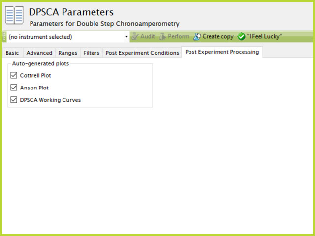
Figure 6. Double Potential Step Chronoamperometry (DPSCA) Post-Experiment Processing Tab in AfterMath
On the Post-Expeirment Processing Tab for DPSCA, users can enable three additional plots: Cottrell Plot (see Figure 7), Anson Plot (see Figure 8), or DPSCA Working Curves (see Figure 9). Tick the checkbox next to the plot to add them to the archive following the completion of the experiment.
Ticking the box next to Cottrell Plot displays a plot of i vs. t-1/2 (see Figure 7). Note that for the Cottrell Plot, the level portion in the plot is actually the time prior to the current spike shown in the chronoamperogram (see Figure 7). That is, earlier time points are to the right in a Cottrell Plot. This is not the case for an Anson Plot because integrating the current with respect to time gives charge.
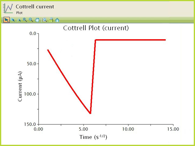
Figure 7. Chronoamperometric (Current) Cottrell Plot of Ferrocene
Ticking the box next to Anson Plot displays a plot of Q vs. t1/2 (see Figure 8). The endpoint in an Anson Plot is the total amount of charge passed during the experiment. Monitoring the charge passed during an experiment is a variant of chronoamperometry called Chronocoulometry (see Figure 8).
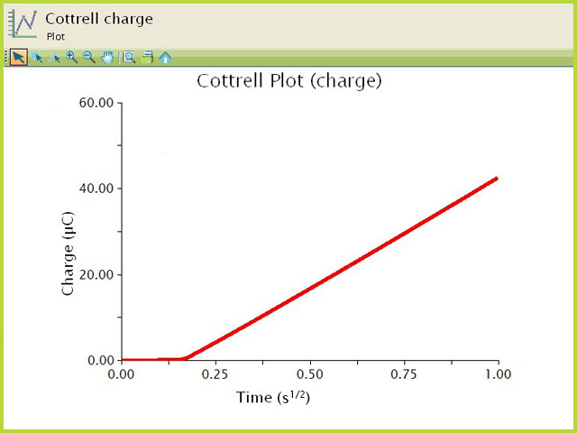
Figure 8. Chronocoulometric (Charge) Anson Plot of Ferrocene
Ticking the box next to DPSCA Working Curves displays a dimensionless plot overlay of actual vs. ideal working curves (see Figure 9). If there are no kinetic complications in the electrode reaction, the actual working curve should fall on an ideal working curve as shown in Figure 9. Note that the deviation at the beginning of the working curve is due to the electronics of the potentiostat.
Dividing the reverse current at time

by

at time

and keeping

allows for the generation of a working curve given by the equation
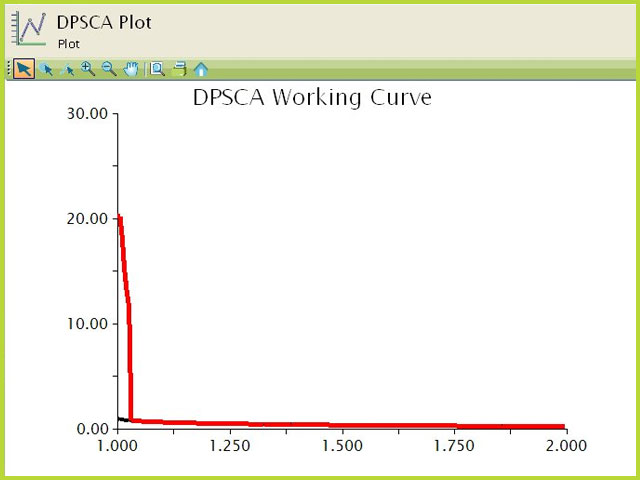
Figure 9. Double Potential Step Chronoamperometry (DPSCA) Working Curve
4Sample Experiment
The results for a 2.5 mM solution of Ferrocene in 0.1 M Bu4NClO4 (MeCN) are shown in Figure 10. The experimental parameters are as follows:
- 2 mm OD Pt working electrode
- forward step potential of 0.75 V vs. Ag/AgCl
- reverse step potential of 0 V vs. Ag/AgCl
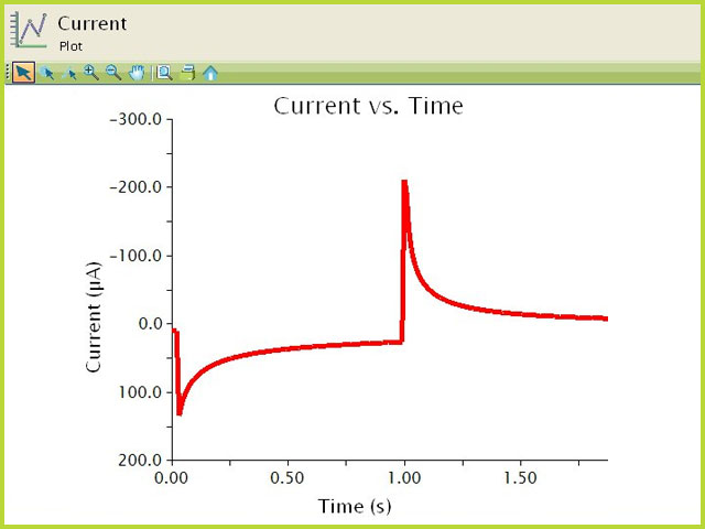
Figure 10. Double Potential Step Chronoamperogram of a Ferrocene Solution
5Example Applications
This example uses DPSCA to calculate the diffusion coefficients for a subtrate

and a product

of an electrode reaction. Hyk et al. examined the current transients for DPSCA to analyze the reaction
.
The researchers generated equations for dealing with both hemispherical electrodes and disk microelectrodes under diffusion-limited and mixed diffusion-migration. Interestingly, the researchers were able to show that for an uncharged substrate with less than 0.1% supporting electrolyte they are able to obtain diffusion coefficients. This is significant because an uncharged substrate with less than 0.1% supporting electrolyte does not lend to calculation of diffusion coefficients by single potential step chronoamperometry.
In another case, Long et al. used a slight variant of DPSCA to examine diffusion and self-exchange in a cobalt bipyridine redox polyether hybrid.
Films of material, containing supporting electrolyte, were prepared on inter-digitated array electrodes (IDAs). A step was generated (equivalent to a double potential step) on one set of IDA electrodes while the current was monitored on the second set IDA electrodes. Monitoring the time it takes for the pulse to travel from the generator to collector electrodes allowed for the calculation of diffusion coefficients and self-exchange rate constants between metal centers.
In the final example, Schwarz and Shain used DPSCA to measure the rate constant for a chemical reaction after an electrochemical reaction, commonly referred to as an EC reaction.
The overall reaction for the general process is
where the product

is electrochemically inactive. In this example, the researchers reduce azobenzene to hydrazobenzene which in turn rearranges to benzidine in acidic solutions. By varying the time of the second step, the researchers were able to determine the rate constant for the reaction of hydrazobenzene rearrangning to benzidine.
Others have used DPSCA to calculate the catalytic rate constant and diffusion coefficient values,
for the qultitfication of bromine and bromide,
, and to monitor diffusion of hydrogen species in the various phases.
6References
-
Bard, A. J.; Faulkner, L. A. Electrochemical Methods: Fundamentals and Applications, 2nd ed. Wiley-Interscience: New York, 2000.
-
Cottrell, F. G. Residual current in galvanic polarization regarded as a diffusiona problem. Z. Phys. Chem., 1903, 42, 385–431.
-
Tomihito, K. Polarographic Diffusion Current Observed with Square Wave Voltage. I. Effect Produced by the Sudden Change of Electrode Potential. Bull. Chem. Soc. Jpn., 1954, 27(8), 523-526.
-
Hyk, W.; Nowicka, A.; Stojek, Z. Direct Determination of Diffusion Coefficients of Substrate and Product by Chronoamperometric Techniques at Microelectrodes for Any Level of Ionic Support. Anal. Chem., 2002, 74(1), 149-157.
-
Long, J. W.; Terrill, R. H.; Williams, M. E.; Murray, R. W. An Electron Time-of-Flight Method Applied to Charge Transport Dynamics in a Cobalt Bipyridine Redox Polyether Hybrid. Anal. Chem., 1997, 69(24), 5082-5086.
-
Schwarz, W. M.; Shain, I. Investigation of First-Order Chemical Reactions Following Charge Transfer by a Step-Functional Controlled Potential Method. The Benzidine Rearrangement1. J. Phys. Chem., 1965, 69(1), 30-40.
-
Hameed, R. M. A. Nickel Oxide Nanoparticles Supported on Graphitized Carbon for Ethanol Oxidation in NaOH Solution. J. Cluster Sci., 2019.
-
Xie, Y.; Cheng, I. F. Selective and rapid detection of triacetone triperoxide by double-step chronoamperometry. Microchem. J., 2010, 94(2), 166-170.
-
Martindale, B. C. M.; Menshyakau, D.; Ernst, S.; Compton, R. G. Room temperature ionic liquid as solvent for in situ Pd/H formation: hydrogenation of carbon–carbon double bonds. PCCP, 2013, 15, 1188-1197.


![\displaystyle -i_r(t)=\frac{nFAD_O^{1/2}C_O^*}{{\pi}^{1/2}} \left[\frac{1}{{(t-\tau)}^{1/2}}-\frac{1}{t^{1/2}} \right]](https://s0.wp.com/latex.php?latex=%5Cdisplaystyle+-i_r%28t%29%3D%5Cfrac%7BnFAD_O%5E%7B1%2F2%7DC_O%5E%2A%7D%7B%7B%5Cpi%7D%5E%7B1%2F2%7D%7D+%5Cleft%5B%5Cfrac%7B1%7D%7B%7B%28t-%5Ctau%29%7D%5E%7B1%2F2%7D%7D-%5Cfrac%7B1%7D%7Bt%5E%7B1%2F2%7D%7D+%5Cright%5D&bg=ffffff&fg=000&s=0&c=20201002)