Ramp Chronopotentiometry (RCP)

Last Updated: 1/5/23 by Alex Peroff

ARTICLE TAGS

chronopotentiometry,
voltage vs. time,
AfterMath RCP,
ramp chronopotentiometry,
RCP

RELATED PRODUCTS

AFTERMATH LINKS

Chronopotentiometry (CP)

Article Contents/Section Navigation

1Technique Overview

Ramp Chronopotentiometry (RCP) is a galvanostatic method in which the current at the working electrode is swept from an initial current to a final current at a set sweep rate. The working electrode potential and current are recorded as a function of time. A plot of working electrode potential versus working electrode current, known as a potentiogram, is produced at the end of the experiment. RCP is the galvanostatic equivalent of cyclic voltammetry (CV).

Ramp Chronopotentiometry (RCP) is an extension of the basic method chronopotentiometry, , where current is swept from an initial to final current at a specified sweep rate. One of the first parameters a user selects is the number of segments.

In the simplest case, when Segments (S_N) = 1, current is swept linearly from an initial to final current, sampling potential at specified intervals (see Figure 1).

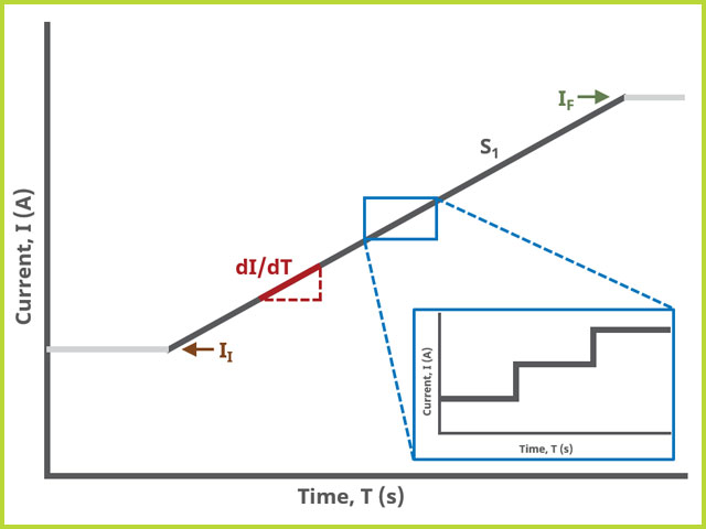
Figure 1. Ramp Chronopotentiometry (RCP) One Segment Waveform

In the simplest case, when Segments (S_N) = 2, current is swept linearly from an initial to vertex current and back to final current, sampling potential at specified intervals (see Figure 2).

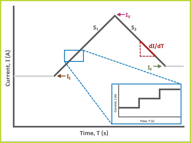
Figure 2. Ramp Chronopotentiometry (RCP) Two Segment Waveform

In the simplest case, when Segments (S_N) ≥ 3, current is swept linearly from an initial to final current with two additional turning points called upper and lower current, sampling potential at specified intervals (see Figure 3). In this case, the most advanced waveform can be designed.

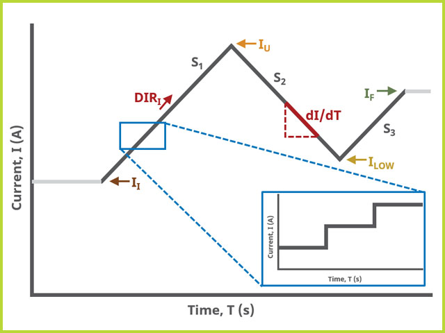
Figure 3. Ramp Chronopotentiometry (RCP) Three Segment Waveform

Over the last few decades, many research reports have emerged using various types of chronopotentiometry, including RCP. Many researchers employ RCP to perform kinetic studies at electrodes and for the elucidation of adsorption mechanisms.

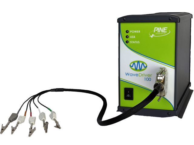
Modern Pine Research potentiostats have digital waveform generators on board. This means that linear sweeps are approximated by a series of small stair steps, whose step size is defined by the 16-bit resolution Analog-to-Digital converter (ADC) on the circuit board and current/potential range selected. For example, on the WaveDriver 100, , the current step resolution on the ±100 nA range is

$\displaystyle \frac{200 \: \text{nA}}{2^{16}}=3.1 \: \text{pA}$

Appropriate current and/or potential filters are automatically employed to "smooth" the jagged edges of this step sequence, enhancing the linearity of the sweep, but can be controlled by the user on the Filters tab of any experiment.

2Fundamental Equations

The following is a very brief introduction to the theory of Ramp Chronopotentiometry (RCP). Consult standard sources for more detailed information.

RCP is a technique that can be utilized to calculate a concentration or a diffusion coefficient (similar to cyclic voltammetry ). Consider a general reaction

$\displaystyle O+e^- \rightarrow R$

with a formal potential E^0'. As current is applied to the working electrode, $O$ begins reducing at the electrode surface, producing $R$ . The potential of the electrode, $E$ , moves to values characteristic of the $O/R$ couple, based on a time-based Nernstian relation. As the concentration of $O$ drops to zero at the electrode surface the potential starts to rapidly increase to more negative values. The resulting E-t curve is much like a potentiometric titration with a transition time (analogous to an equivalence point), $\tau$ . 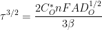The potential at one-half $\tau$ is E^0'. The transition time is related to the concentration and diffusion coefficient of $O$ through the expression

$\displaystyle \tau^{3/2} = \frac{2C_O^*nFAD_O^{1/2}}{3\beta}$

where $C_O^*$ is the concentration of $O$ (mol/cm³), $n$ is the number of electrons, $F$ is Faraday’s Constant (96,485 C/mol), $A$ is the electrode area (cm²), $D$ is the diffusion coefficient (cm²/s) and $\beta$ is the sweep rate (A/s). For rapid electrode kinetics, the time-based Nernstian equation is

$\displaystyle E=E_{\tau /4}+\frac{RT}{nF}\ln{\frac{{\tau}^{1/2}-t^{1/2}}{t^{1/2}}}$

where $E_{{\tau}/4}$ is equal to

$\displaystyle E_{\tau /4} = E^{0'} - \frac{RT}{2nF}\ln{\frac{D_O}{D_R}}$

Finally, plotting $E \: \text{vs.} \: \ln{\frac{{\tau}^{1/2}-t^{1/2}}{t^{1/2}}}$ shows a straight line with a slope of $RT/nF$ for a reversible $E-t$ curve.

3Experimental Setup in AfterMath

To perform a ramp chronopotentiometry (RCP) experiment in AfterMath, choose Ramp Chronopotentiometry (RCP) from the Experiments menu (see Figure 4).

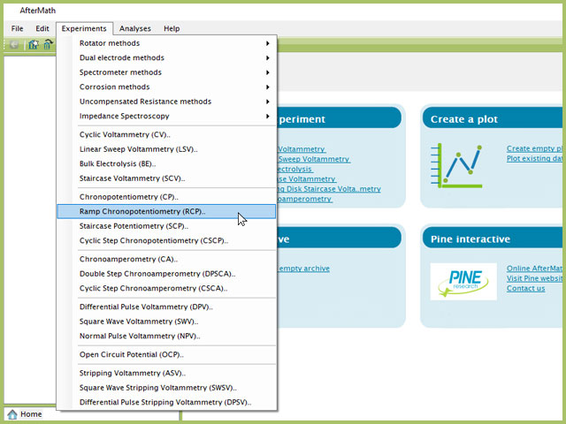
Figure 4. Ramp Chronopotentiometry (RCP) Experiment Menu Selection in AfterMath

Doing so creates an entry within the archive, called RCP Parameters. In the right pane of the AfterMath application, several tabs will be shown (see Figure 5).

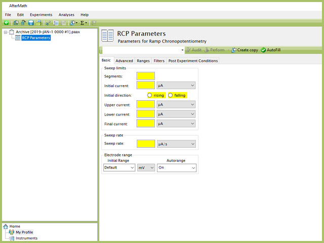
Figure 5. Ramp Chronopotentiometry (RCP) Expeirment in AfterMath

As with most Aftermath methods, the experiment sequence is

Induction Period → Electrolysis Period → Relaxation Period → Post-Experiment Idle Conditions

Like many experiments, the Induction and Relaxation Periods are on the Basic Tab. The parameters for a CP experiment are fairly simple compared to other methods in AfterMath.

3.1Basic Tab

TIP: Click the AutoFill button ("I Feel Lucky" prior to May 2019) on the top bar in AfterMath to automatically fill all required parameters with reasonable starting values. While the values provided may not be appropriate for your specific system, they are reasonable parameters with which to start your experiment, especially if you are new to the method.

The basic tab contains fields for the fundamental parameters necessary to perform an RCP experiment. AfterMath shades fields with yellow when a required entry is blank and shades fields pink when the entry is invalid (see Figure 3).

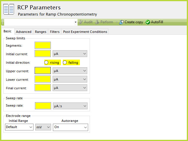
Figure 3. Ramp Chronopotentiometry (RCP) Experiment Basic Tab in AfterMath

During the induction period, a set of initial conditions are applied to the electrochemical cell and the cell equilibrates at these conditions (set on the Advanced Tab). Data are not collected during the induction period, nor are they shown on the plot during this period.

After the induction period, the current applied to the working electrode is swept to the next specified value (based on segments) for the duration of the experiment, which is called the sweep period. The galvanostatic circuit of the instrument maintains constant applied current while simultaneously measuring the potential at the working electrode relative to the reference electrode. During the electrolysis period, potential and current at the working electrode are recorded at regular intervals as specified on the Advanced Tab.

The experiment concludes with a relaxation period. During the relaxation period, a set of final conditions (specified on the Advanced tab) are applied to the electrochemical cell and the cell equilibrates at these conditions (set on the Advanced Tab). Data are not collected during the induction period, nor are they shown on the plot during this period.

A plot of the typical experiment sequence, containing labels of the fields on the Basic tab, helps to illustrate the sequence of events in an RCP experiment (see Table 1 and Figure 4).

The table below lists the group and field names and symbol for each parameter associated with this experiment (see Table 1).

Group Name	Field Name	Symbol
Sweep	Segments	$S_N$
Sweep	Initial Current	$I_I$
Sweep	Initial Direction	$DIR_I$
Sweep	Upper Current	$I_U$
Sweep	Vertex Current	$I_V$
Sweep	Lower Current	$I_{LOW}$
Sweep	Final Current	$I_F$
Sweep	Sweep Rate	$dI/dT$

Table 1. Basic Tab Group Names, Field Names, and Symbols.

Figure 4. Ramp Chronopotentiometry (RCP) Three Segment Waveform Field Diagram

RCP is one of several methods in AfterMath where users can specify the number of Segments (S_N) that will be used in the waveform. As described in Section 1 above, there are different fields used based on the number entered into the Segments field. When S_N ≥ 2, Vertex Current field is shown on the Basic Tab. When S_N ≥ 3, Vertex Current field is replaced with Upper Current and Lower Current fields on the Basic tab.

The Electrode Range group on the Basic Tab is used to specify the expected potential and/or current range to use on the experiment. For RCP, potential is the measured valued and as such, users can select the most appropriate potential range from the dropdown menu. The most appopriate range is the one that completely includes the expected potential spread across the entire experiment, but it not significantly greater.

Some instruments, such as the WaveNow series, feature only one potential range (e.g., ±10 V for the WaveNow^XV ) whereas other potentiostats have multiple potential ranges (e.g., ±2.5 V, ±10 V, and ±15 V for the WaveDriver 100 ). Note that the selection is only choosing the initial range. If Autorange is not Off, then as data are collected, AfterMath will choose the most appropriate range as needed (if there is more than one). If Autorange is Off, and the initial range is too small, then potential may go off scale and the results will be truncated. If the intial potential range is too large, and Autorange is Off, then the data may have a noisy, choppy, or quantized appearance. More on the topic of Electrode Range is provided elsewhere in the knowledgebase.

At the end of the relaxation period, the post-experiment idle conditions are applied to the cell, and the instrument returns to the idle state. The default plot generated from the data is measured potential vs. time, called a chronoamperogram.

3.2Advanced Tab

The RCP Advanced tab contains groups for Induction Period, Relaxation Period, iR Compensation, and Sampling (see Figure 5).

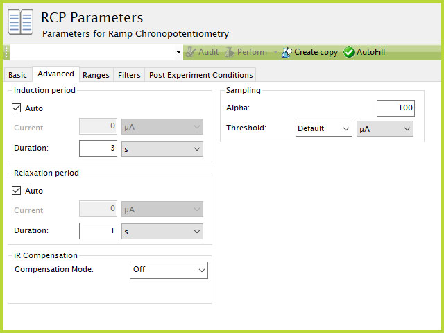
Figure 5. Ramp Chronopotentiometry (RCP) Experiment Advanced Tab in AfterMath

Induction Period is the first step in an RCP experiment if the Duration is >0 s. During the induction period, the specified current is applied to the cell for the specified duration. During this period, data are not collected. The Induction Period is believed to "calm" the cell prior to intentional perturbation. More on Induction Period is found within the knowledgebase.

Relaxation Period is the last step in an RCP experiment if the Duration is >0 s. During the relaxation period, the specified current is applied to the cell for the specified duration. During this period, data are not collected. The Relaxation Period is believed to "calm" the cell after intentional perturbation. More on Relaxation Period is found within the knowledgebase.

Detailed description of the iR Compensation Mode is provided elsewhere on the knowledgebase. This mode is used to correct for uncompensated resistance in the electrochemical cell.

The Sampling group defines the potential sampling rate for the experiment There are two parameters in this group, Alpha and Threshold. As mentioned previously, digital instruments (such as the WaveNow and WaveDriver series potentiostats) approximate a linear sweep with a series of tiny steps.

As shown, alpha is the total time after each small step, from 0% to 100% and the value of alpha defines the time at which a sample is measured (see Figure 6). If $\alpha=0$ , potential is measured immediately after the small step. If $\alpha=100$ then potential is measured just before the next small step. In general, it is recommended to measure sweep experiments at $\alpha=100$ , which is the default setting.

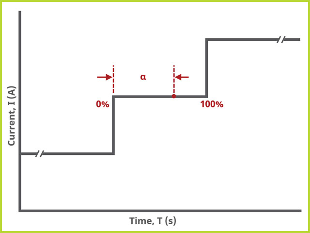
Figure 6. Galvanostatic Approximation of a Linear Sweep (Micro View)

The threshold defines the frequency of sampling. There are two options from the dropdown which are "Default" and "None." Additionally, a specific current interval can be added by typing a numeric value into the dropdown box and selecting the appropriate units. Briefly, the options can be described as follows:

Default. This setting will use the default settings, which are 5 mV for potentiostatic experiments and 1 µA for galvanostatic experiments.
None. This setting will enable collection of the maximum number of data points possible. The value is not easily known, as is a combination of the sweep rate and sweep limits. Choose this option to collect the maximum number of data points that the hardware can acquire.
Manual entry. In this case, type an integer value into the dropdown menu and select the appropriate units in the next dropdown menu. For example, a user may only wish to collect a data point every 20 mV or every 100 µA, in which case these are entered into the fields.

NOTE: Not all threshold values, manually entered, will be allowed. The software will use the value provided and match as closely to it as possible. The actual sampling rate may be higher, exact, or lower than the value entered. Presently, AfterMath will not inform you of the threshold value actually possible, but it can be inferred after the completion of the experiment and viewing the time-based data stream, where the threshold can be calculated as the time difference between data points.

NOTE: Archive file size increases as the threshold decreases. In other words, a smaller interval means more data will be collected per experiment whereas a larger interval means fewer data will be collected per experiment. For long-term experiments, Pine Research recommends the default threshold, unless users require a finer level of detail per sweep.

3.3Ranges, Filters, and Post Experiment Conditions Tab

In nearly all cases, the groups of fields on the Ranges tab are already present on the Basic tab. The Ranges tab shows an Electrode Range group and depending on the experiment shows either, or both, current and potential ranges and the ability to select an autorange function. The fields on this tab are linked to the same fields on the Basic tab (for most experiments). Changing the values on either the Ranges tab or on the Basic tab changes the other set. In other words, the values selected for these fields will always be the same on the Ranges tab and on the Basic tab. More on ranges is found within the knowledgebase, as is for autorange.

The Filters tab provides access to potentiostat hardware filters, including stability, excitation, current response, and potential response filters. Pine Research recommends that users contact us for help in making changes to hardware filters. Advanced users may have an easier time changing the automatic settings on this tab. Filter settings fields are shown for WK1 (working electrode #1) as well as for WK2 (working electrode #2) regardless of the potentiostat connected to AfterMath.

By default, the potentiostat disconnects from the electrochemical cell at the end of an experiment. There are other options available for what these post-experiment conditions can be and are controlled by setting options on the Post Experiment Conditions tab.

4Typical Results

Typical RCP results for a solution of ferrocene are shown (see Figures 7-8). By default, AfterMath produces a chronopotentiogram that is potential vs. current (see Figure 7). Under Other Plots → Potential, the raw potential vs. time plot is available (see Figure 8). For the data presented below, the experimental parameters were as follows:

2 mM ferrocene in 0.1 M Bu₄NClO₄ (MeCN)
2 mm OD platinum working electrode
platinum counter electrode
Ag/AgCl reference electrode
1 µA/s sweep rate

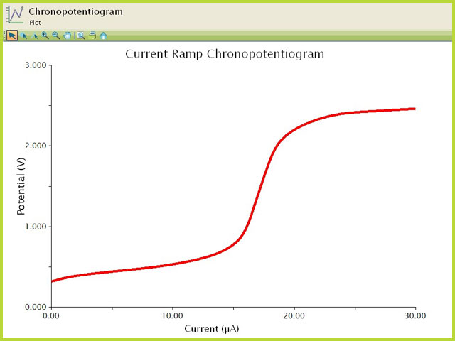
Ramp Chronopotentiogram of 2 mm Ferrocene (Potential vs. Current)

Figure 7. Ramp Chronopotentiogram (RCP) of 2 mm Ferrocene (Potential vs. Current)

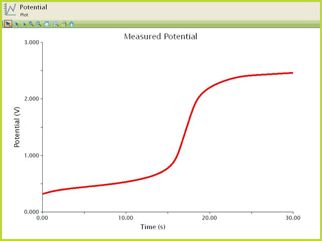
Figure 8. Ramp Chronopotentiogram (RCP) of 2 mm Ferrocene (Potential vs. Time)

How can we help? What do you want to learn? Search our knowledgebase.

Galvanostatic Methods

Ramp Chronopotentiometry (RCP)

ARTICLE TAGS

RELATED PRODUCTS

RELATED PAGES

AFTERMATH LINKS

Article Contents/Section Navigation

1Technique Overview

2Fundamental Equations

3Experimental Setup in AfterMath

3.1Basic Tab

3.2Advanced Tab

3.3Ranges, Filters, and Post Experiment Conditions Tab

4Typical Results

5References

Questions? Find Answers.

Software

Applications

Theory

Product Specifications