


EIS Data Accuracy and Validity
Last Updated: 1/4/23 by Alex Peroff
1Conditions of EIS Data
Prior to analysis of EIS data, it is critical to consider how potentiostat limits may affect the accuracy of results. All commercial potentiostats have calibrated internal hardware (and often external hardware, like the cell cable, as well), but there are always physical limitations on the range of conditions an instrument can accurately measure. The user should consult the potentiostat’s accuracy contour plot (ACP), which is a half-Bode plot
 Bode Plot
illustrating the accuracy limits of measured
Bode Plot
illustrating the accuracy limits of measured  over a wide range of frequencies, to evaluate data accuracy, particularly at high frequencies where the accuracy becomes substantially reduced.
over a wide range of frequencies, to evaluate data accuracy, particularly at high frequencies where the accuracy becomes substantially reduced.In addition to the physical limitations of the potentiostat being used to collect EIS data, there are other factors to consider related to data accuracy and validity. While an AC signal (potential or current waveform) can be physically applied to almost any electrochemical system, it is not guaranteed that the resulting data may be accurately classified as “impedance”. There are three primary conditions that must be met during an EIS experiment for the results to be considered valid impedance data:
- Stability - the electrochemical system must not change with respect to time, and it must return to its initial state without further oscillations once the applied signal is terminated
- Causality - the resultant signal must only be caused by, and be solely a function of, the applied signal
- Linearity - the resultant signal must exhibit a linear response to the applied signal; or, the resultant signal must obey the law of superposition with respect to the input signal; or, the measured impedance of the resultant signal must be independent of the magnitude of the applied signal amplitude
1.1Stability
One strategy for maintaining stability is to allow sufficient settling time at the EIS setpoint before applied sinusoidal signals begin. Enough time must be allowed for the system to reach steady-state before collecting EIS data, otherwise there may be drift in the baseline that leads to unsteady and erroneous EIS data. Effect of drift is also more pronounced at lower frequencies due to the extended time required to complete slower sine waves (see Figure 1 for effect of drift on sinusoidal signals and Figure 2 for effect on Lissajous plots).
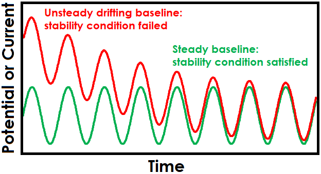
Figure 1. Drifting Baseline Effect on Sinusoidal EIS Waveform
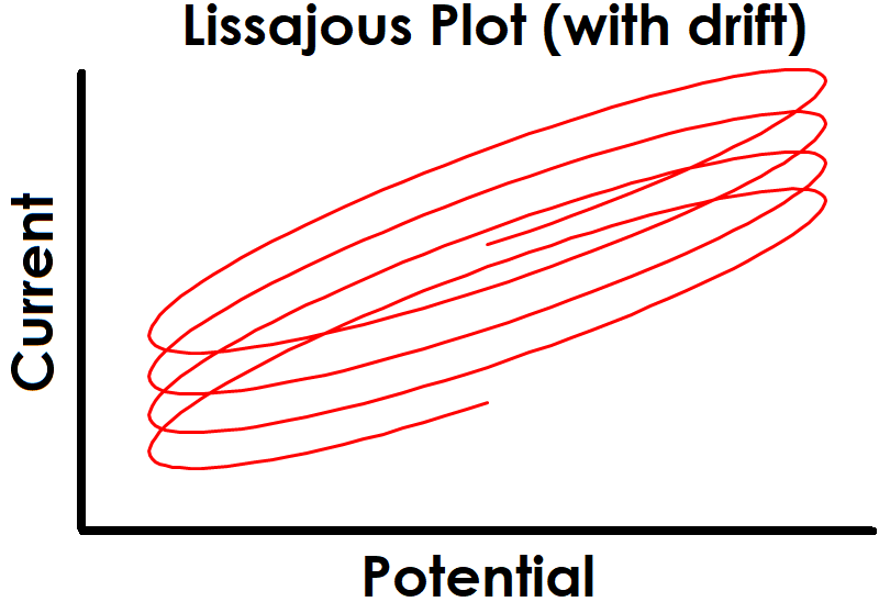
Figure 2. Drifting Baseline Effect on EIS Lissajous Plot
Often, the EIS setpoint is chosen as the open circuit potential. In these cases, the system may not need much extra time to reach a stable condition since it may already be at open circuit during idle periods before running the EIS experiment. When applying sinusoidal signals on top of a potential or current setpoint, however, lack of sufficient settling time can lead to erroneous data. Additionally, since most commercial potentiostats automatically perform an OCP measurement during EIS experiments, switching between setpoint and OCP just prior to applied sinusoidal signals may interrupt the stability of an electrochemical system. When possible, a final settling period placed between the OCP step and applied sinusoidal signals should be added to prevent baseline drift.
1.2Causality
Causality is a difficult condition to determine practically. It can be tricky to know definitively whether the electrochemical response during an EIS experiment is solely a result of the applied signal. One way to indirectly infer causality is to observe the system response, if any, once the applied sinusoidal signals have completed (see Figure 3 for examples of both potentially causal and non-causal cases). While it is not absolute evidence of a lack of causality, observing continued noise or oscillations after the signal has been discontinued may cast doubt on whether the electrochemical signal was influenced by other sources or general system instability.
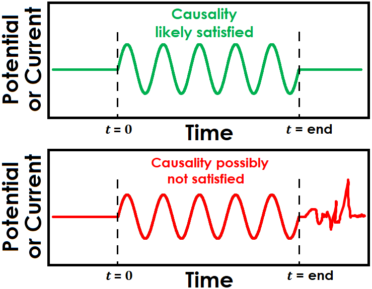
Figure 3. Illustration of EIS Causality Condition
1.3Linearity
The condition of linearity is often satisfied by taking precautions with respect to the amplitude of an EIS experiment. For example, even though the average electrochemical system is entirely nonlinear, it may be considered roughly linear over a narrow potential window. It is therefore commonplace for the applied signal amplitude to be very small (around 5 - 20 mV for potentiostatic EIS) to ensure linearity. However, it is also important that the applied signal is large enough to properly induce a measurable response for the potentiostat to monitor. This creates a balancing act to find the optimal range of applied signal amplitudes: large enough to adequately excite the system but small enough to maintain linearity. Typically, trial-and-error is the most effective way to clarify this range and determine the desirable experimental parameters for a given electrochemical system.
As this optimal amplitude is elucidated during experimentation of EIS parameters, another check on linearity can be done by observing the ratio of input and output amplitudes. For example, if the input amplitude is doubled and the output amplitude does not also double, the linearity condition is not likely satisfied.
Finally, perhaps the most obvious indication of a lack of linearity can be quickly determined by the shape of the Lissajous plot. Figure 4 shows examples of Lissajous plots for linear systems, and examples of distorted Lissajous plots from nonlinear systems are shown in Figure 5. Some commercial software packages display Lissajous plots as they occur live during an EIS experiment. In these cases, the user can rapidly determine if the system is displaying nonlinear behavior and cancel the test if necessary.
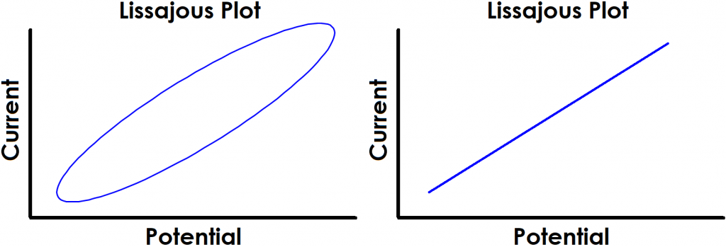
Figure 4. Examples of Typical Lissajous Plots for Linear Systems
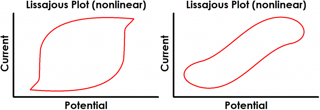
Figure 5. Examples of Typical Lissajous Plots for Nonlinear Systems