EIS Basic Background Theory

Last Updated: 1/4/23 by Alex Peroff

ARTICLE TAGS

EIS,
eis theory,
eis fundamental

Related Products

Related AfterMath Entries

AfterMath Downloads

Article Contents/Section Navigation

1Theory

A cursory introduction to theory and concepts related to electrochemical impedance spectroscopy is presented herein. For a more thorough and complete study, the reader is encouraged to consult academic textbooks and the scientific literature.

Experimental electrochemistry can be as powerful as it is tricky. Even simple DC methods (e.g., voltammetry, open circuit potential, chronoamperometry, chronopotentiometry) are often plagued by inaccuracies and/or poor signal-to-noise ratios resulting from seemingly insignificant or overlooked sources. Variables that can affect electrochemical data include, but are not limited to: the state and quality of electrodes, electrolyte, experimental hardware, the physical laboratory layout, software experimental parameters, arrangement of cables, and grounding configuration.

AC techniques, like electrochemical impedance spectroscopy (EIS), can be similarly affected by these variables and sources of error. The user must exercise particular care and caution when setting up and running EIS experiments as the impact of small sources of error often has a larger effect on data quality than for DC methods. Obtaining and interpreting meaningful EIS data, as with many other facets of electrochemistry, requires repeated practice and often some trial-and-error with respect to both the hardware and software.

In AC electrochemistry, a sinusoidal potential (or current) signal is applied to a system and the resulting current (or potential) signal is recorded and analyzed (see Figure 1 for diagram and Table 1 for associated terminology). The frequency and amplitude of the input signal are tuned by the user, while the output signal normally has the same frequency as the input signal but its phase may be shifted by a finite amount.

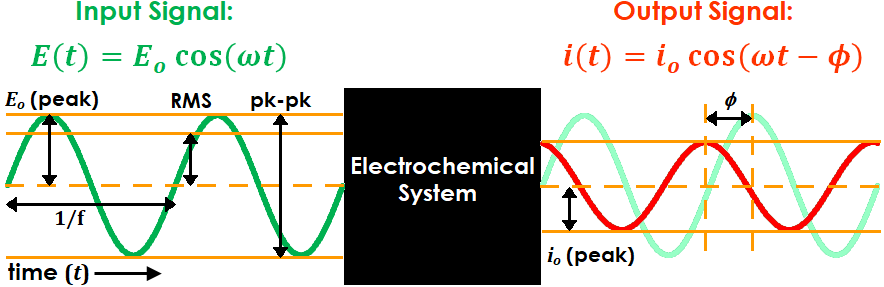
EIS Sine Wave Input and Output Terminology

Figure 1. AC Electrochemistry Sine Wave Input and Output Terminology

Symbol	Definition
$\displaystyle{E(t)}$	time-dependent potential
$\displaystyle{E_o}$ (peak)	peak potential amplitude
RMS	root mean square potential amplitude
pk-pk	peak-to-peak potential amplitude
$\displaystyle{t}$	time
$\displaystyle{i(t)}$	time-dependent current
$\displaystyle{i_o}$ (peak)	peak current amplitude
$\displaystyle{\phi}$	phase angle
$\displaystyle{f}$	frequency (units of Hz)
$\displaystyle{\omega}$	angular frequency (units of rad/s)

Table 1. AC Electrochemistry Input and Output Symbol Definitions

Practically, frequency (f) is reported in units of Hz. However, for mathematical convenience the angular frequency (ω), which has units of rad/s and is equivalent to 2πf, is typically used for calculations instead (e.g., see input and output signal equations in Figure 1). Similarly, the phase angle ( $\displaystyle{\phi}$ ) is typically reported in units of degrees but calculated in units of radians.

There are three conventions often used to define the input (and sometimes output) signal amplitude: peak, peak-to-peak, and RMS. “Peak” refers to the difference between the sine wave set point (i.e., the potential or current at the beginning of the sine wave period) and its maximum or minimum point (i.e., the potential or current at one quarter of the sine wave period). “Peak-to-peak” is simply twice the peak value (see Figure 1).

“RMS”, which stands for “root mean square”, is a mathematical quantity used primarily in electrical engineering to compare AC and DC voltages or currents. Though its practical relevance and importance to EIS measurements is somewhat minimal, it is still widely used in the industry to characterize input signal amplitude. Mathematically, it is equivalent to the peak value divided by $\displaystyle{\sqrt{2}}$ , or roughly peak times 0.707 (see Figure 1).

During an EIS experiment, a sequence of sinusoidal potential signals with varying frequencies, but similar amplitudes, is applied to an electrochemical system. Typically, frequencies of each input signal are equally spaced on a descending logarithmic scale from ~10 kHz - 1 MHz to a lower limit of ~10 mHz - 1 Hz. Application of these input and output signals is usually performed automatically via a potentiostat/galvanostat.

Monitoring the progress of an EIS experiment can be done by observing the input and output signals on a single current vs. potential graph called a Lissajous plot (see Figure 2). Depending on the system under study, as well as the applied frequency and amplitude, the shape of the resulting Lissajous plot may vary. Throughout an EIS experiment, the user can observe the progression and pattern of Lissajous plots as a means of identifying possibly erroneous data.

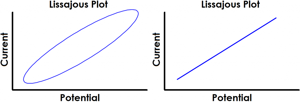
EIS Lissajous Plots for Stable and Linear Systems

Figure 2. Examples of Typical Lissajous Plots for Stable and Linear Systems

The shape of the current vs. potential Lissajous plot for a stable, linear electrochemical system typically appears as either a tilted oval or straight line that repeatedly traces over itself (see Figure 2). The width of the oval is indicative of the magnitude of the output signal phase angle. For example, if the Lissajous plot looks like a perfect circle, it means the output signal is completely out of phase (i.e., +90°) with respect to the input signal. This is also the EIS response experienced by an ideal capacitor or inductor.

How can we help? What do you want to learn? Search our knowledgebase.

EIS Theory

EIS Basic Background Theory

ARTICLE TAGS

Related Products

Related Pages

Related AfterMath Entries

Article Contents/Section Navigation

1Theory

2References

Questions? Find Answers.

Software

Applications

Theory

Product Specifications