Uncategorized – Page 23 – Pine Research Instrumentation Store

This article is part of the AfterMath Data Organizer Electrochemistry Guide.

Chronoamperometry is a technique where the potential of the working electrode is stepped for a specified period of time. Current is plotted as a function of time. Chronoamperometry is also known as potential step amperometry.

Detailed Description

Like most of the other electrochemical techniques offered by the AfterMath software, this experiment begins with an induction period. During the induction period, a set of initial conditions is applied to the electrochemical cell and the cell is allowed to equilibrate to these conditions. The default initial condition involves holding the working electrode potential at the initial potential for a brief period of time (i.e., 3 seconds). After the induction period, the potential of the working electrode is stepped to a specified potential for a period of time. After the step has finished, the experiment concludes with a relaxation period. The default condition during the relaxation period involves holding the working electrode potential at the initial potential for an additional brief period of time (i.e., 1 seconds). At the end of the relaxation period, the post experiment idle conditions are applied to the cell and the instrument returns to the idle state.

Current is plotted as a function of time, resulting in a chronoamperogram. You may also choose to do some post experiment processing in order to generate a Cottrell plot.

Parameter Setup

The parameters for this method are arranged on various tabs on the setup panel. The most commonly used parameters are on the Basic tab. Additional tabs for Ranges and post experiment idle conditions are common to all of the electrochemical techniques supported by the AfterMath software. Finally, a Post Experiment Processing tab deals with manipulating the data automatically when the experiment is finished.

Basic Tab

You can click on the “I Feel Lucky” button (located at the top of the setup) to fill in all the parameters with typical default values (see Figure 1). You will no doubt need to change the Potential and Hold time in the Forward step period box to values which are appropriate for the electrochemical system being studied. You may also want to change the Number of intervals in the Sampling Control box.

Figure 1: Basic Chronoamperometry Setup

The Electrode Range on the Basic tab is used to specify the expected range of current. If the choice of electrode range is too small, actual current may go off scale and be truncated. If the electrode range is too large, the chronoamperogram may have a noisy, choppy, or quantized appearance.

Some Pine potentiostats (such as the WaveNow and WaveNano portable USB potentiostats) have current autoranging capability. To take advantage of this feature, set the electrode range parameter to “Auto”. This allows the potentiostat to choose the current range “on-the-fly” while the chonoamperogram is being acquired.

The waveform that is applied to the electrode is a simple pulse to the Potential listed in the Forward step period box. Note that the actual waveform that is measured (see Figure 2, red trace) fluctuates slightly compared to the applied potential (see Figure 2, black trace).

Figure 2: Waveform for CA. Black trace = applied potential, Red trace = measured potential.

Ranges Tab

AfterMath has the ability to automatically select the appropriate ranges for voltage and current during an experiment. However, you can also choose to enter the voltage and current ranges for an experiment. Please see the separate discussions on autoranging and the Ranges Tab for more information.

Post Experiment Conditions Tab

After the Relaxation Period, the Post Experiment Conditions are applied to the cell. Typically, the cell is disconnected but you may also specify the conditions applied to the cell. Please see the separate discussion on post experiment conditions for more information.

Post Experiment Processing Tab

The Post Experiment Processing Tab (see Figure 3) allows you to automatically generate Cottrell current or Cottrell charge plots. Please see the Typical Results and Theory sections of this wiki for more information regarding Cottrell plots.

Figure 3: Post Experiment Processing Options.

Typical Results

The results for a $2 mM$ solution of ferrocene in $0.1 M Bu_4NClO_4/MeCN$ are shown in Figure 4.

Figure 4: Chronoamperogram of a ferrocene solution using a potential = $0.75 V vs. Ag/AgCl (aq)$ and a $2 mm$ Pt WE.

If you selected to automatically generate Cottrell plots, the plots are under the other plots folder in the Archive navigation panel. Choosing Cottrell current displays a plot of $i\;vs. t^{-1/2}$ (see Figure 5A). Choosing Cottrell charge displays a plot of $Q \;vs. t^{-1/2}$ (see Figure 5B). Note that for the Cottrell Current plot, the level portion in the plot is actually the time prior to the current spike shown in Figure 4. That is, earlier time points are to the right in a Cottrell Current Plot. This is not the case for a Cottrell Charge plot because integrating the current with respect to time gives charge. The endpoint in a Cottrell Charge plot is the total amount of charge passed during the experiment. Monitoring the charge passed during an experiment is a variant of chronoamperometry called Chronocoulometry. See the Applications section for an example of Chronocoulometry.

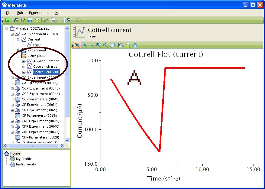
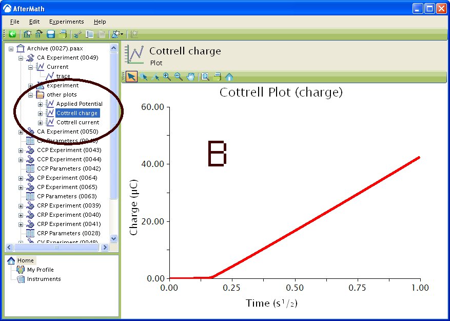
Figure 5 : Post experiment processing plots. A – Cottrell Current $(i)$ , B – Cottrell Charge $(Q)$ . Conditions as listed in Figure 4.

The Cottrell current plot is a useful diagnostic tool to examine that your species of interest is freely diffusion in solution. Upon applying the potential step, the current initially spikes, then begins trail off. As will be explained in more detail in the Theory section, the current during the trailing off period is a diffusion-limited current dictated by the Cottrell equation. Examining the Cottrell Current plot in this region reveals that the current is linear with respect to $t^{-1/2}$ (see black ellipse in Figure 6).

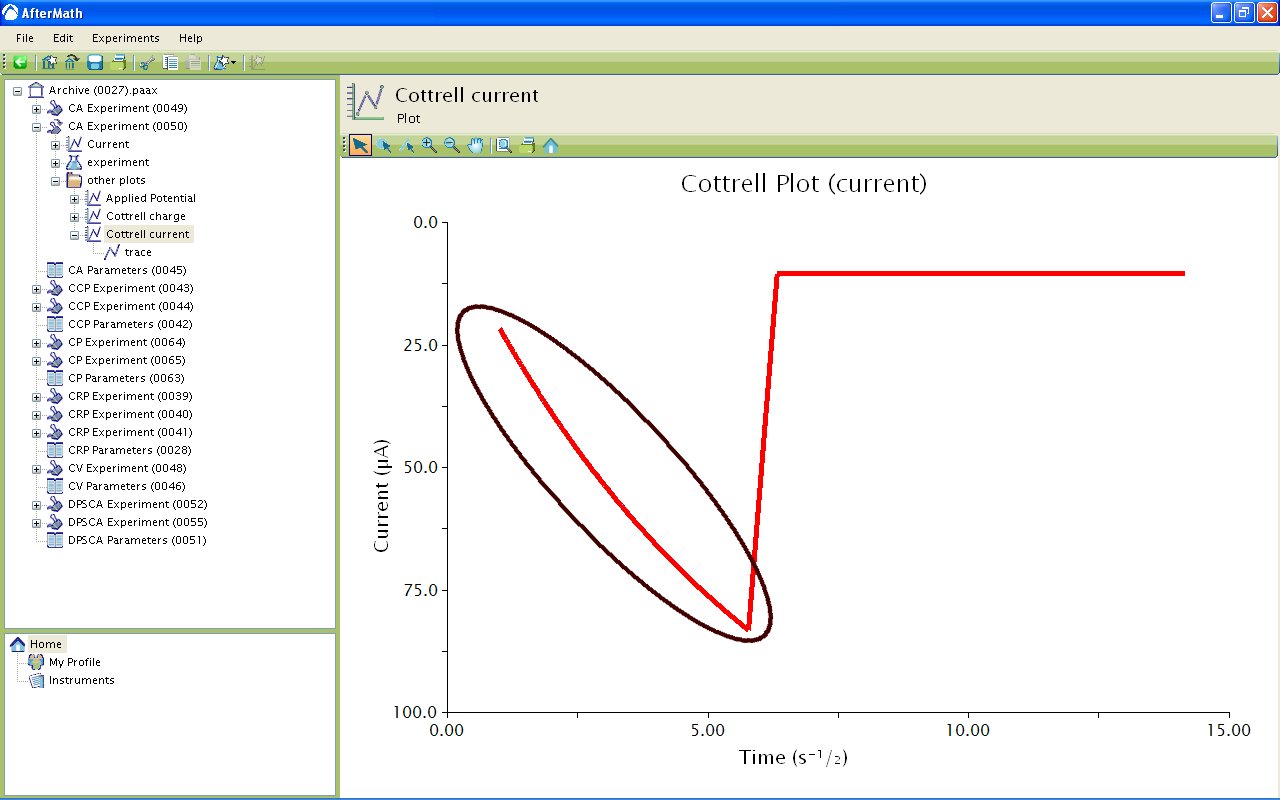
Figure 6: Highlight of Diffusion-limited Current in Cottrell Current Plot.

The addition of a Baseline tool to the diffusion limited current region allows for calculation of the diffusion coefficient for the species of interest if the concentration and electrode area are known (see Figure 7). First you will have to delete the region of the Cottrell Plot where current is not diffusion limited. Use the Point Selection Tool to delete the unwanted points of the Cottrell Plot. Next, add a baseline tool by right clicking on the leftover point and select Add Tool » Baseline. Manipulate the control points to provide an adequate fit. AfterMath automatically provides the slope and intercept for the Baseline tool.

Figure 7: Addition of Baseline Tool in Diffusion-limited Current Region.

The slope of the line in the plot is given by the equation

$slope={\frac{nFAD_O^{1/2}C_O^*}{{\pi}^{1/2}}}$

where $n$ is the number of electrons, $F$ is Faraday’s Constant $(96485 C/mol)$ , $A$ is the electrode area $(cm^2)$ , $D_O$ is the diffusion coefficient $(cm^2/s)$ , and $C$ is the concentration $(mol/cm^3)$ . In the example above, $D$ is calculated to be $1.6{\times}10^{-5}cm^2/s$ .

Theory

The theory section is split into two segments. The first segment deals with Chronoamperometry (CA) and the second section deals with Chronocoulometry (CC). Chronoamperometry leads to Chronocoulometry natually since charge is obtained by integrating current with respect to time.

Chronoamperometry

The following is a basic description of the theory behind Chronoamperometry. Please see the literature¹ for a more detailed description of the technique. Consider a reaction $O+e\;{\rightleftharpoons}\;R$ with a formal potential $E^{{\circ}'}$ . In general, the potential step applied to the working electrode should be sufficiently more negative than $E^{{\circ}'}$ such that reduction of $O$ to $R$ is complete at the surface of the electrode (i.e. surface concentration of $O$ at the electrode surface is $0$ ). When this occurs, the current is diffusion-limited, much like the current that flows in CV after the potential of the electrode sweeps past $E_p$ .

When the current is diffusion-limited in CA, the current-time response is described by the Cottrell² equation
$i=\frac{nFAD_O^{1/2}C_O^*}{({\pi}t)^{1/2}}&s=3$ where $n$ is the number of electrons, $F$ is Faraday’s Constant $(96485 \:C/mol)$ , $A$ is the electrode area $(cm^2)$ , $D_O$ is the diffusion coefficient $(cm^{2}/s)$ , and $C_O^*$ is the concentration $(mol/cm^3)$ . As described in the Typical Results section, plotting $i \;vs. t^{-1/2}$ gives a slope that contains the diffusion coefficient, $D$ .

Chronocoulometry

The following is a brief description of chronocoulometry. Please see the literature¹ for a more detailed description of the technique. Chronocoulometry is advantages in some ways over chronoamperometry. First is that the signal grows with time, meaning that the later portion of the experiment are least distorted by the nonideal potential rise, giving better signal-to-noise ratios. Second, integrating smooths random noise making the data cleaner. Third, contributions from double-layer charging and reactions of adsorbed species can be separating from those of freely diffusion species. The cumulative charge passed during the experiment is given by the equation

$Q_d={\frac{2nFAD_O^{1/2}C_O^*t^{1/2}}{\pi^{1/2}}}$

where the parameters are as described in the above section. Typically, a plot of $Q \;vs.\; t^{-1/2}$ has a non-zero y-intercept. This intercept is related to double-layer charging and reduction of adsorbed $O$ . The overall equation describing the charge is then given by

$Q_d={\frac{2nFAD_O^{1/2}C_O^*t^{1/2}}{\pi^{1/2}}}+Q_{dl}+nFA\Gamma_O$

where $Q_{dl}$ is the charge due to double-layer charging and $nFA\Gamma_O$ is the charge due to reduction of adsorbed $O$ . $Q_{dl}$ and $nFA\Gamma_O$ are not easily separated and usually require additional experiments such as double potential step chronoamperometry. However, approximations for $Q_{dl}$ can be made by performing the same potential step in a solution of only electrolyte. This is only an approximation because the true double-layer charging will be influenced by adsorbed $O$ .

The Application section in the next tab contains examples of both Chronoamperometry and Chronocoulometry.

Application

In the first example, Tennyson et al.³ used chronoampometry to determine the diffusion coefficients (D) and number of electrons (n) for a series of indirectly connected bimetallic complexes. In this instance, the researchers used microelectrodes to generate steady-state currents. Plotting of the function

${\frac{i(t)}{i_{ss}}}$ $vs.$ $t^{-1/2}$

allows for the calculation of $D_O$ without knowledge of $C_O^*$ or $n$ . Though the experiments are relatively simple and straightforward, the researchers then used these values for more complicated electrochemical experiments that enabled them to determine the degree of electronic coupling between the two metallic centers. Understanding the degree of electronic coupling could allow for facilitation to otherwise inaccessible catalysts and materials.

The next example uses chronoamperometry to measure extremely small diffusion coefficients of redox polyether hybrid cobalt bipyridine molten salts. Crooker and Murray⁴ performed chronoamperometry on a series of undiluted molten salts and were able to obtain diffusion coefficients as low as $10^{-17} cm^2/s$ . The researchers went on to obtain heterogeneous rate constants $(k^0)$ using CV and were able to show that the reaction remains quasireversible despite small $k^0$ rates because $D_O$ values are so low.

The next example uses chronoamperometry to directly measure rate constants. Smalley et al.⁵ examined a series of monolayers terminated with either a ferrocene or ruthenium redox moiety. For monolayers containing more than 11 methylene units, chronoamperometry was used to determine the heterogeneous rate constants $(k^0)$ . The researchers also determined preexponential factors and found them to be much lower that expected based aqueous solvent dynamics.

The fourth example uses chronocoulometry. Wolfe et al.⁶ prepared a series of ferrocenated hexanethiolate protected Au nanoparticles. Normallly, TGA would be used to calculate the number of thiolates per nanoparticle. However, in this case, TGA was inconclusive due to a slow loss of mass over the applied temperature range. The researchers instead monitored the charge pass over time for solution of nanoparticles with known concentrations. Knowing the total charge passed and the particle concentration allowed them to determine the number of ligands per nanoparticle. This is a good example of how electrochemistry can be used in place of a more traditional characterization technique.

The final example also uses chronocoulometry, but rather than using it for quantification purposes, the researchers use it to evoke a change in the system. Zhang et al.⁷ use chronocoulometry with predefined endpoints to produce Ag nanoparticles, confined on a electrode surface, with varying shapes and sizes. By varying the amount of charge passed the researchers were able to show that triangular nanoparticles oxidize first on the bottom edge, followed by triangular tips, followed by out-of-plane height. Since the researchers also coupled spectroscopy to their electrochemical experiments they were also able to show how the SPR band changes with shape evolution. This is a nice example of how electrochemistry can be used to evoke a change in a system rather than simply to monitor changes or determine physical parameters of the system.

References

Additional Resources

Links

This article is part of the AfterMath Data Organizer Electrochemistry Guide

Rotating disk bulk electrolysis (BE-RDE) is very similar to bulk electrolysis (BE) in that a constant current or constant potential is applied to a two or three compartment electrochemical cell in order to effect a large change in the oxidation state of an analyte. The amount of charge passed during the electrolysis can be calculated by integrating the current with respect to time. In almost any bulk electrolysis experiment, the solution is stirred in some way. The unique aspect of the method discussed here (BE-RDE) is that a rotating electrode is used both to stir the electrode and to convey the analyte towards the electrode surface.

Detailed Description

Like most of the other electrochemical techniques offered by the AfterMath software, this experiment begins with an induction period. During the induction period, a set of initial conditions is applied to the electrochemical cell and the cell is allowed to equilibrate to these conditions. The default initial condition involves holding the working electrode potential at the Initial Potential for a brief period of time (i.e., 3 seconds). If the potentiostat is being used to control the rotator speed, the rotator is also spun at the desired speed during this time. The WaveNow and WaveNano are capable of outputting a potential proportional to the desired rotator speed. This output can then be coupled to the input on an MSR rotator for fully automated control of the rotation speed.

Bulk electrolysis can be used to impart a large electrochemical change on a system. This can be complete oxidation or reduction or a species, the complete production of a product through electrochemical synthesis or just a partial oxidation or reduction of a compound to change the ratio of oxidized and reduced species.

Bulk electrolysis typically consists of a three chamber electrochemical cell with the chambers separated by glass frits. One chamber has the working electrode, which is the rotating electrode in this case. The second chamber usually has the reference electrode and the third chamber houses the auxiliary electrode.

After the induction period, a potential is applied to the cell for the specified period of time. After electrolysis the conditions specified in the relaxation period are applied to the cell.

Finally, the Post Experiment Conditions are applied to the cell.

The results of an electrolysis are usually presented as a plot of current versus time. Integrating the current versus time data produces a plot of charge versus time.

Parameter Setup

The parameters for this method are arranged on various tabs on the setup panel. The most commonly used parameters are on the Basic tab, and less commonly used parameters are on the Advanced tab. Additional tabs for Ranges and post experiment idle conditions are common to all of the electrochemical techniques supported by the AfterMath software.

Basic Tab

The Basic Tab (see Figure 1) contains parameters related to the Induction period, Electrolysis period, Relaxation period, Electrode range and Sampling control.

Some Pine potentiostats (such as the WaveNow and WaveNano portable USB potentiostats) have current and voltage autoranging capabilities. To take advantage of this feature, set the Electrode range parameter to “Auto”. This allows the potentiostat to choose the current and voltage ranges “on-the-fly” while the electrolysis is conducted. Please see the wiki regarding Electrode Range for a more detailed description and example of how the integrity of the data is affected by the choice of the range.

Typically, the Induction period, Relaxation period, and Sampling control parameters are filled in. You must enter a Potential and Duration for the electrolysis.

The Number of intervals in the Sampling control box is the number of data points taken during the experiment. A larger number of intervals means that the number of data points acquired will be more and data files will therefore be larger. Likewise, a smaller intervals means that fewer points will be acquired and data files will be smaller.

Figure 1: Basic setup for rotating disk controlled potential bulk electrolysis.

The waveform that is applied to the electrode first starts with the potential entered in the Induction period, followed by the potential entered in the Electrolysis period, and finally followed by the potential entered in the Relaxation period (see Figure 2).

Figure 2 : Waveform applied to electrode throughout experiment

The Electrode Range on the Basic tab is used to specify the expected range of current. If the choice of electrode range is too small, actual current may go off scale and be truncated. If the electrode range is too large, the current-time curve may have a noisy, choppy, or quantized appearance. Please see the ugly duckling webpage for an example of what happens when an improper range is selected.

Finally, the Rotation Parameters box contains the Speed parameter. Even if the potentiostat is not being used to control the rotator, you must enter a rotation speed.

Post Experiment Conditions Tab

Typical Results

In the typical result discussed below, the starting material, $K_4Fe(CN)_6$ , is partially oxidized to $K_3Fe(CN)_6$ by applying a sufficiently positive potential ( $+500 mV$ ) to drive the oxidation. The end result of the experiment is a mixture of $K_4Fe(CN)_6$ and $K_3Fe(CN)_6$ .

Prior to performing the electrolysis, the observed value of the open circuit potential ( $~50 mV$ ) was consistent with a solution containing primarily the reduced form of the analyte, $K_4Fe(CN)_6$ . In addition, a preliminary cyclic voltammogram (see Figure 3, experimental parameters: $K_4Fe(CN)_6$ in $0.1 \; M \; Na_2SO_4$ , $2 \; mm$ Pt disc working electrode, Pt counter electrode, sweep rate $100 \; mV/s$ ) confirms that a significant oxidation current is observed if the working electrode potential is at or above $500 \; mV$ .

Figure 3: Cyclic voltammogram of a Potassium Ferrocyanide Solution

The principle result from a bulk electrolysis is a plot of current versus time (see Figure 4, experimental parameters: $K_4Fe(CN)_6$ in $0.1 \; M \; Na_2SO_4$ , $5 \; mm$ Pt Disk, $2800 \; rpm$ , Pt mesh counter electrode, Electrolysis Potential = $0.5 V$ ). Integrating the current with respect to time will yield total charge ( $Q$ ) passed during the experiment. One way to accomplish this integration is to use the Area Tool. This tool can be added to a trace with a right-click on the trace followed by choosing Add Tool » Area from the menu. Once the tool is placed on the trace, you can manipulate the control points to choose the limits of the integration (see Figure 5). In this example, the total charge ( $Q$ ) passed during the electrolysis is $26.96 \; mC$ .

Figure 4: Bulk electrolysis of a Potassium Ferrocyanide Solution

Figure 5 : Using the control points to manipulate the area tool

Finally, the open circuit potential measured after the electrolysis period is $0.275 \; V$ . The ratio of oxidized to reduced species can then be calculated using the Nernst equation shown below

$E = E^{0'} + \frac{RT}{nF} ln \left(\frac{[K_3Fe(CN)_6]}{[K_4Fe(CN)_6]}\right)$

where $E$ is the open circuit potential, $E^{0'}$ is the formal potential ( $0.230 \; V$ in this instance), $R$ is the Universal Gas Constant, $T$ is the absolute temperature, $n$ is the number of electrons and $F$ is the Faraday Constant ( $96485 \; C/mol$ ). The ratio of oxidized to reduced species in this example is $5.77:1$ , meaning that the solution contains approximately $85\% \; K_3Fe(CN)_6$ and $15\% \; K_4Fe(CN)_6$ .

For a complete electrolysis example, consult the basic discussion of bulk electrolysis (BE).

Theory

The theory of bulk electrolysis is really quite simple. However, for a more thorough description of the technique and general considerations, you are directed to the literature.¹

Consider a reaction $O + e^- \rightarrow R$ , where $O$ is reduced to $R$ in a one electron reaction. A solution of $m$ moles of $O$ would require $m$ moles of electrons to completely reduce $O$ to $R$ . Upon applying a sufficient reducing potential, a large amount of $O$ is converted to $R$ and subsequently swept away from the electrode by stirring. As more $O$ is converted to $R$ the current falls off exponentially until it reaches background level. It is at this point, the electrolysis can be stopped. The charge ( $Q$ ) passed during the experiment can be obtained by integrating the current with respect to time.

$Q = {\int}i(t) \; dt$

The charge can then be converted to the number of moles of $O$ using the equation

$m = \frac{Q}{Fn}$

where $F$ is Faraday's constant, and $n$ is the number of electrons transferred during the reaction.

Application

The first instance of BE-RDE reduced $Cu(II)$ onto a copper disk electrode. Puglisi and Bard² utilized BE-RDE to remove most of the stirring noise associated with traditional electrolysis. Also, the authors were able to calculate a diffusion coefficient from the coulometric current-time curve that matched well with a value obtained using RDE.

One recent application highlights the usefulness of BE using RDE. Chardon-Noblat et al.³ synthesized a the macromolecule $[Ru(bpy)(MeCN)_2Cl_2]$ in a one-electron reduction of a $Ru(III)$ precursor. Previously, this molecule was only obtained in mixtures with the corresponding tris(acetonitrile) derivative, $[Ru(bpy)(MeCN)_3Cl]$ . The authors also chemically synthesize the $[Ru(bpy)(MeCN)_2Cl_2]$ using a one-electron reducing reagent, sodium diethyldithiocarbamate. Correlating the amount of charge passed during electrolysis with the amount of liberated chloride ion confirmed that the electrochemical synthesis of the desired complex proceeded with no side reactions. This application highlights the usefulness of bulk electrolysis for synthesis.

For more typical applications, please see the Application section of regular BE.

References

1. Faulkner, L. R.; Bard, A. J. Bulk Electrolysis Methods, Electrochemical Methods: Fundamentals and Applications, 2^nd ed.; Wiley: New Jersey, 2000; 417-470.

2. Puglisi, V. J.; Bard, A. J. Anal. Lett. 1970, 3, 443-448.

3. Chardon-Noblat, S.; Renfrew, A.; Lafolet, F.; Deronzier, A.; Jakonen, M.; Laurila E.; Haukka, M. Dalton Trans. 2008, 5891-5896.

Additional Resources

Links: Electrochemist's Guide, AfterMath User's Guide, AfterMath Main Support Page

Related Techniques: Bulk Electrolysis, Dual Electrode Bulk Electrolysis

Posted 1/4/2016 in Uncategorized

This article is part of the AfterMath Data Organizer Electrochemistry Guide

Bulk Electrolysis is a technique where either a constant current or constant potential is applied to an two or three comparment electrochemical cell in order to effect a large change in the oxidation state of a species of interest. The amount of charge passed during the electrolysis can be calculated by integrating the current with respect to time.

Synonyms: Controlled Potential Electrolysis, Potentiostatic Coulometry, Controlled Potential Coulometry,

Detailed Description

The basic setup for Controlled Potential Bulk Electrolysis is shown in Figure 1. Bulk electrolysis can be used to impart a large electrochemical change on a system. This can be complete oxidation or reduction or a species, the complete production of a product through electrochemical synthesis or just a partial oxidation or reduction of a compound to change the ratio of oxidized and reduced species.

Bulk electrolysis typically consists of a three chamber electrochemical cell with the chambers separated by glass frits. One chamber has the working electrode. This chamber should be stirred to provide maximum mass transport to the electrode during electrolysis. The second chamber usually has the reference electrode and the third chamber houses the auxiliary electrode. Note that both the working and auxiliary electrodes should have a large surface area (typically platinum meshes or vitrious carbon).

After the induction period, a potential is applied to the cell for the specified period of time. After electrolysis the conditions specified in the relaxation period are applied to the cell.

Finally, the Post Experiment Conditions are applied to the cell.

Current is plotted as a function of time which can be integrated to yield total charge passed during electrolysis.

Parameter Setup

The parameters for this method are arranged on the two tabs of the setup panel. The parameters relating to bulk electrolysis are on the Basic tab and the post experimental parameters are on the Post experiment conditions tab.

Basic Tab

The Basic Tab (see Figure 1) contains parameters related to the Induction period, Electrolysis period, Relaxation period, Electrode range and Sampling control.

Typically, the Induction period, Relaxation period, and Sampling control parameters are filled in. You must enter a Potential and Duration for the electrolysis.

Figure 1: Basic setup for controlled potential bulk electrolysis.

Figure 2 : Waveform applied to electrode throughout experiment

Post Experiment Conditions

Typical Results

In the typical result discussed below, $K_4Fe(CN)_6$ was oxidized to $K_3Fe(CN)_6$ by the application of a potential of $0.57 \;V$ . The purpose of the experiment was to convert $Fe^{2+}$ in the complex to $Fe^{3+}$ . A cyclic voltammogram of the solution is shown below to show that the potential of $0.57 \; V$ will oxidize completely $K_4Fe(CN)_6$ (see Figure 3, a $2 \; mm$ Pt disc working electrode and Pt counter electrode were used with a sweep rate of $100 \; mV/s$ ).

Figure 3 : Cyclic Voltammogram of a Potassium Ferrocyanide Solution

The principle result from a bulk electrolysis is a plot of current versus time (see Figure 4, experimental conditions were: $5 \; mL$ of $K_4Fe(CN)_6$ in $0.1 \; M \; KCl$ , Pt mesh working electrode, Pt mesh counter electrode, Electrolysis Potential $= 0.57 V$ ). Integration of current with respect to time will yield total charged ( $Q$ ) passed during the experiment.

Figure 4 : Bulk Electrolysis of a Potassium Ferrocyanide Solution.

Right-click on the trace to bring up a dialog box and choose Add Tool » Area in order to integrate the area under the curve (see Figure 5).

Figure 5 : Add Area Tool to electrolysis results

You can manipulate the control points of the tool in order to obtain a proper area under the curve (see Figure 6).

Figure 6 : Drawing the proper baseline

The total charge ( $Q$ ) passed during electrolysis was $459.0 \; mC$ or $0.459 C$ . This charge can then be used to calculate the number of moles of species in solution through the use of Faraday's Constant ( $F, \; 96485 \; C/mol$ ) using the equation below:

$m = \frac{Q}{Fn}$

where $n$ is the number of electrons for the redox process. $F$ and $Q$ are defined above. The number of moles of
$K_4Fe(CN)_6$ in solution was $4.76$ x $10^{-6}$ . Dividing this by the volume of solution ( $4 \; mL$ in this instance) in the cell, yields a concentration of $1.19$ x $10^{-3} \; M$ .

Theory

The theory of bulk electrolysis is really quite simple. However, for a more thorough description of the technique and general considerations, please see the literature.¹

$Q = \int i(t) dt$

The charge can then be converted to the number of moles of $O$ using the equation

$m = \frac{Q}{Fn}$

where $F$ is Faraday's constant, and $n$ is the number of electrons transferred during the reaction.

Application

Four examples of the usefulness of bulk electrolysis are shown below.

The first example shows has bulk electrolysis can be used to quantify the amount of a species in solution. Wolfe and coworkers² electrolyzed solutions of gold nanoparticles passivated with a layer of 6-(ferrocenyl) hexanethiol. Typically, quantitation of the number of ligands protecting a nanoparticle is accopmlished through the use of thermogravimetric analysis (TGA). However, since ferrocene sublimes easily, TGA was inconclusive. The researchers were able to quantitate the number of ligands by using solutions of known nanoparticle concentration and oxidizing ferrocene to ferrocenium. By determining the charge passed during the experiment, they were able to calculate the number of ligands per nanoparticle. This first example is useful because it shows that an electrochemical technique such as bulk electrolysis can be used in places whether traditional techniques might fail.

The second example uses bulk electrolysis to deposit a film of cobalt-based water oxidation catalysts. Surendranath and coworkers³ oxidized $Co^{2+}$ to $Co^{3+}$ in the presence of various electrolyte solutions. $Co^{3+}$ reacts with the electrolytes, forming a thin film of particles on an ITO electrode. Complete electrolysis of the solution was not necessary to form the films that were later used as water oxidation catalysts. This second example is useful since it illustrates that bulk electrolysis need not be solely used to completely oxidize or reduce a species in solution. Rather, the partial electrolysis was enough for the researchers to make their thin films.

The third example shows how bulk electrolysis can be used in a chemical synthesis. Blattes and coworkers⁴ used bulk electrolysis to simultaneously generate cycloaddition partners for inverse-electron demand Diels-Alder reactions. Inverse-electron demand Diels-Alder reactions have not been used as extensively as the normal Diels-Alder reaction due to the limited availability of readily accessible simple electron-deficient dienes. Using bulk electrolysis, the researchers were able to access, in situ, two unstable entities for use in cycloaddition reactions. The researchers were even able to show regiospecificity and diastereospecificity in the case of heterocyclic annulations.

Finally, the fourth example shows how bulk electrolysis can be used to teach electrochemisty to first-year undergraduate students. Chyan and Chyan⁵ used screen-printed electrodes to examine the metal-deposition process through bulk electrolysis. Normally, electrochemistry is introduced at a later time in the undergraduate curriculum when students have had more time to develop essential lab skills. Since the electrodes are screen printed the usually labor-intensive step of electrode preparation is removed. Using a variety of deposition solutions, students are able to generate films of different, visually-attractive films in one lab period. Along with the introduction of Faraday's Law, the researchers are also able to introduce electrodeposition efficiency since these electrodes can be weighed after the deposition process. This great example shows a wonderful way to get students hooked on the fascinating world of electrochemistry.

References

1. Faulkner, L. R.; Bard, A. J. Bulk Electrolysis Methods, Electrochemical Methods: Fundamentals and Applications, 2^nd ed.; Wiley: New Jersey, 2000; 417-470.

2. Wolfe, R. L.; Balasubramanian, R.; Tracey, J. B.; Murray, R. W. Langmuir, 2007, 23, 2247–2254.

3. Surendranath, Y.; Dinca, M.; Nocera, D. G. J. Am. Chem. Soc., 2009, 131, 2615–2620.

4. Blattes, E.; Fleury, M.-B.; Largeron, M. J. Org. Chem., 2004, 69, 882-890.

5. Chyan, Y.; Chyan, O. J. Chem. Educ. 2008, 85, 565.

Additional Resources

Links: Electrochemist's Guide, AfterMath User's Guide, AfterMath Main Support Page

Posted 1/4/2016 in Uncategorized

Owners of the Pine CBP Bipotentiostat system who are presently using our classic PineChem software may wish to upgrade to our new AfterMath software package. Such an upgrade is likely to involve both a software upgrade and a corresponding hardware upgrade. This article discusses some of the issues to consider when contemplating an upgrade.

What can I get for free?

All users of our classic PineChem software may take advantage of the FREE AfterMath Viewer download option. If you are only looking for the ability to analyze data and prepare plots from your bipotentiostat data, then you can download a free copy of our AfterMath Viewer software package. The viewer permits you to import PineChem data files directly into the AfterMath viewer software, and then you can prepare plots and analyze data using AfterMath.

AfterMath Download

What if I want to control the CBP Bipotentiostat using AfterMath?

If you wish to to control your CBP Bipotentiostat using AfterMath, then you need to consider upgrades to all five of the following components in your existing CBP system:

Interface Board Upgrade. The interface board (which is installed inside the computer) must be a 16-bit interface board. Older bipotentiostat systems are likely to have an earlier 12-bit interface board rather than a 16-bit interface board. Because AfterMath uses the interface board to digitally generate the waveform applied to the working electrode, it is essential to use a higher resolution 16-bit interface board when working with AfterMath. If you have purchased your CBP bipotentiostat system recently, you may already have a 16-bit interface board. If not, you will need to purchase a 16-bit board (click here for details)
Filter Board Upgrade. When using the interface board to send digital waveforms to the bipotentiostat and to record the response from the potentiostat, it is very likely that noise will be introduced as signals travel between the computer and the bipotentiostat. For this reason, Pine strongly recommends that a signal filter board be installed in the bipotentiostat. This easily installed add-on board provides various levels of signal filtering for both the excitation signals and the response signals travelling in the interface cable. (click here for details)
Software License Upgrade. The software license for AfterMath is tied to the particular interface board installed in the computer. For this reason, it is important to first settle the issue of the 16-bit interface board upgrade (discussed above) before ordering AfterMath from Pine. You will need to report the serial number of your interface board to Pine at the time you purchase the AfterMath upgrade (click here for details)
Operating System Upgrade. AfterMath works with Windows 8, Windows 7, Windows Vista, and Windows XP (32 bit). If you are using a computer with an earlier version of Windows, then you will need to upgrade the operating system. (click here for minimum system requirements)
Device Driver Upgrade. If you upgrade the interface board and/or the operating system, then you will very likely need to upgrade the device driver for the interface board. (click here for device driver information)

How much does it cost to upgrade?

Pine is happy to provide you with a quotation for an upgrade package. Contact Pine at (919) 782-8320 or using our online contact form (click here). We will be happy to help you evaluate exactly what you need to successfully upgrade your system.

In general, most customers choose to purchase the filter board together with the software license directly from Pine. In the event that an interface board upgrade is also required, Pine can also supply the interface board, but it is generally less expensive to purchase the interface board directly from National Instruments.

What features does AfterMath offer?

AfterMath software has many advantageous features. In each of the tabs below, the functions of the software are displayed.

Classic PineChem

Data Analysis and Plotting Features
Multi-Trace Overlay Plotting
Peak Area, Height & Baseline Tools
Trace Data Transform Functions
Drag-n-Drop Traces on to Plots
Full Support for SI Units
Select Traces, Segments, and Points
International Unicode Font Support
Superscripts, Subscripts, Symbols
Publication Quality Printing
Queueing Multiple Experiments
Control of Multiple Potentiostats
Cell Control while Idle

System Clipboard Support
Copy Trace Data to Clipboard
Copy Trace Data from Clipboard
Copy Plot Image to Clipboard

Original PineChem Methods:
Cyclic Voltammetry (CV)
Bulk Electrolysis (BE)
– Constant Potential
Dual Electrode Cyclic Voltammetry (DECV)
– Collection, Shielding, and Window variants
Dual Electrode Bulk Electrolysis (DEBE)
– Controlled Potential

Additional Single Step Methods:
Open Circuit Potential vs time (OCP)
Bulk Electrolysis (BE)
– Constant Current
Dual Electrode Bulk Electrolysis (DEBE)
– Mixed Mode Constant Current and/or Potential
Single-Step Chronoamperometry (CA)

Staircase, Pulse, and Multistep Methods:
Double-Step Chronoamperometry (DPSCA)
Linear Staircase Voltammetry (LSCV)
Differential Pulse Voltammetry (DPV)
Square Wave Voltammetry (SWV)
Normal Pulse Voltammetry (NPV)
– including Reverse Normal Pulse Voltammetry

Cyclic Staircase & Pulse Methods:
Cyclic Staircase Voltammetry (CSCV)
Cyclic Differential Pulse Voltammetry (CDPV)
Cyclic Square Wave Voltammetry (CSWV)
Cyclic Normal Pulse Voltammetry (CNPV)
– including Cyclic Reverse Normal Pulse Voltammetry

Galvanostatic Methods:
Chronopotentiometry (CP)
Current Ramp Chronopotentiometry (CRP)
Cyclic Current Ramp Potentiometry (CCP)

Stripping Voltammetry (anodic and cathodic):
Stripping Voltammetry (ASV)
Differential Pulse Stripping Voltammetry (DPSV)
Square Wave Stripping Voltammetry (SWSV)

Data Storage Formats
PineChem Setup File (.stp)
PineChem Results File (.exp)
AfterMath Data Archive (.paax)

Limited
Limited
Limited
No
No
No
No
No
No
No
No
Yes

No
No
No

Yes
Yes
Yes
Yes
Yes
Yes
Yes

No
No
No
No
No
No

No
No
No
No
No
No

No
No
No
No
No

No
No
No

No
No
No

Yes
Yes
No

AfterMath – Viewer Only Version

System Clipboard Support
Copy Trace Data to Clipboard
Copy Trace Data from Clipboard
Copy Plot Image to Clipboard

Galvanostatic Methods:
Chronopotentiometry (CP)
Current Ramp Chronopotentiometry (CRP)
Cyclic Current Ramp Potentiometry (CCP)

Stripping Voltammetry (anodic and cathodic):
Stripping Voltammetry (ASV)
Differential Pulse Stripping Voltammetry (DPSV)
Square Wave Stripping Voltammetry (SWSV)

Data Storage Formats
PineChem Setup File (.stp)
PineChem Results File (.exp)
AfterMath Data Archive (.paax)

Yes
Yes
Yes
Yes
Yes
Yes
Yes
Yes
Yes
No
No
Yes

Yes
Yes
Yes

No
No
No
No
No
No
No

No
No
No
No
No
No

No
No
No
No
No
No

No
No
No
No
No

No
No
No

No
No
No

Import Only
Import Only
Yes

AfterMath – Full Version

System Clipboard Support
Copy Trace Data to Clipboard
Copy Trace Data from Clipboard
Copy Plot Image to Clipboard

Galvanostatic Methods:
Chronopotentiometry (CP)
Current Ramp Chronopotentiometry (CRP)
Cyclic Current Ramp Potentiometry (CCP)

Stripping Voltammetry (anodic and cathodic):
Stripping Voltammetry (ASV)
Differential Pulse Stripping Voltammetry (DPSV)
Square Wave Stripping Voltammetry (SWSV)

Data Storage Formats
PineChem Setup File (.stp)
PineChem Results File (.exp)
AfterMath Data Archive (.paax)

Yes
Yes
Yes
Yes
Yes
Yes
Yes
Yes
Yes
Yes
Yes
Yes

Yes
Yes
Yes

Yes
Yes
Yes
Yes
Yes
Yes
Yes

Yes
Yes
Yes
Yes
Yes
Yes

Yes
Yes
Yes
Yes
Yes
Yes

Yes
Yes
Yes
Yes
Yes

Yes
Yes
Yes

Yes
Yes
Yes

Import Only
Import Only
Yes

Download Options

PineChem owners can purchase the full version of AfterMath.

Purchase AfterMath Upgrade

Alternatively, PineChem owners can download the AfterMath Viewer for free.

Free AfterMath Viewer

Posted 1/4/2016 in Uncategorized

This article is part of the AfterMath Data Organizer Electrochemistry Guide

The choice of measurement sensitivity is very important when performing an electrochemical technique. If the instrument sensitivity is set too low, then small signals may be lost in the noise. If the instrument sensitivity is adjusted too high, then even relatively small signals may overwhelm the measurement circuitry, causing large features in the signal to be “clipped” or truncated.

In almost every electrochemical technique, the software is able to automatically choose the proper sensitivity for the excitation signal. For example, before a cyclic voltammetry experiment even begins, the software is well aware that the potential excitation waveform is a simple triangle wave that will alternate between a few known setpoints. Because the magnitude of these setpoints is known ahead of time, the software can automatically match the proper potential measurement sensitivity to these known setpoint levels. Such “software autoranging” is always possible for whichever signal (potential or current) is the excitation signal.

Choosing the proper range for measuring response signals is a bit trickier. the autoranging feature for response signals, when available, is generally done in “real time” by the instrument itself. During an experiment, the instrument actively monitors the response signal levels and makes “on the fly” adjustments to the range settings. For example, in a cyclic voltammetry experiment, the current generally starts off at some small level. Then, as the potential is swept toward the formal potential for an electroactive substance in the cell, the current begins to increase quickly. The instrument senses this increase in current and automatically switches to a less sensitive current range to prevent the ever-growing current signal from being “clipped”.

The advantage to having an instrument capable of autoranging response signals is that you don't need to specify the signal sensitivity ahead of time. The instrument determines the proper range while the experiment is occurring. The disadvantage of such instrument-based autoranging is that small glitches may be introduced into your results whenever the instrument switches from one measurement range to another. These glitches are caused by a momentary loss of cell control during the circuit switching event.

In the worst case, the proper choice of current or potential measurement sensitivity must be determined by a trial-and-error process. By repeating the same experiment once or twice, you are able to determine the anticipated signal levels and adjust the instrument sensitivity accordingly.

The choice to use autoranging for the potential and current signals is made on the Ranges Tab (see above). By default, both of these range settings are set to “Auto”, meaning that the software and/or instrument will attempt to choose an appropriate signal sensitivity automatically.

Not all instruments support the autoranging feature for response signals. For instruments which do not support this feature, choosing the “Auto” range setting usually causes the least sensitive range setting to be selected.

Links: Electrochemist's Guide, AfterMath User's Guide, AfterMath Main Support Page

Related Topics: specifying ranges

Posted 1/4/2016 in Uncategorized
Read More

Security Issues

The Legacy NIDAQ device drivers used with the Pine AFCBP1 Bipotentiostat typically work without any problems when they are installed from an account which has administrative privileges and when the AfterMath or PineChem software applications are run from an account which has administrative privileges.

Problems are encountered, however, when normal user accounts are used to install NIDAQ or to run the AfterMath or PineChem software applications. Typically, customers at large organizations with central control of computing resources are the first to encounter these problems (because such customers do not have access to the administrative accounts on their laboratory computers).

There are ways to overcome these problems if a person with an administrative account is available to assist with the initial installation of the NIDAQ device driver. This article describes Pine's recommendations about how to install AfterMath and NIDAQ in an environment where everyday users will not have access to an administrative account.

Installation

Installation of AfterMath, PineChem and/or the NIDAQ device drivers should ALWAYS be performed using an account with administrative privileges.

Installation is generally a simple matter of downloading the appropriate software (or using an installation CD-ROM), and then running the “setup.exe” file in the installation package. See the AfterMath Installation Guide or NIDAQ Installation Guide for more information.

Instructions for downloading NIDAQ are provided at the end of this article.

Post-Installation NIDAQ Tuning

NOTE: The information in this section is based on National Instruments KnowledgeBase article 3CQGAFHS which has the title ”How Do I Give Non-Administrators Full Control Over National Instruments Products?”.

After the main installation using an administrative account has been completed successfully, the next step is to make sure that all users (both administrators and non-administrators) have access to the folders in which the National Instruments applications were installed. These folders are all typically located within the parent folder “C:Program FilesNational Instruments” (see below).

Note that the following steps should be performed while you are still logged into an administrative account.

Locate the parent National Instruments folder (see below):

Go to the Properties dialog box associated with the parent folder (see below):

Select the “Security” tab, click on the group called “Users”, and then check the box to allow “Full Control” over the folder (see below):

Click the “OK” button after making the changes described above.

At this point, log out of the administrator account and then log into one of the normal user accounts. Launch AfterMath from the normal user account. After a few seconds, AfterMath should detect the presence of the AFCBP1 bipotentiostat connected to the system.

Download

The required NIDAQ device driver (for the interface board) may be downloaded directly from the National Instruments web site.

Device Driver Download

Posted 1/4/2016 in Uncategorized

A complete CBP bipotentiostat system is a combination of the bipotentiostat itself, an interface board and cable (manufactured by National Instruments), and a Windows-based desktop computer (usually provided by the customer). With any system made up of components from a variety of manufacturers, it is important to assure that all of the components are working together in the best possible configuration. In the specific case of the CBP bipotentiostat, a common issue is making sure that the interconnections between the components are made in such a way that excess signal noise is not introduced into the system. This article describes best practices for electrical connections (to eliminate most signal noise at its source) and for signal filtering (for removing noise as the signals are sampled).

Ground Connections

When working with the CBP bipotentiostat system, it is very important to make certain that all parts of the system are properly grounded. The computer system, the monitor, and the bipotentiostat should all be connected to the same grounded power source (i.e., do not connect the computer and the bipotentiostat to different power circuits).

The metal chassis of the bipotentiostat is connected to the earth ground via the third prong on the power cord. The front panel of the bipotentiostat has a convenient binding post (in the lower right corner) that can be used to make additional earth grounding connections as needed. Typically, any metal object located near the electrochemical cell (such as a rotating disk electrode, a clamp holding the cell, or a Faraday cage around the cell) should be connected to the earth ground.

Cell Cable Shielding

The various cables which connect the bipotentiostat to the electrochemical cell should be of the shielded (coaxial) type whenever possible. These cell cables should be routed well away from any power cords, network cables, or video monitors, all of which are considerable sources of electrical noise.

The cable which connects to the reference electrode must be of the shielded coaxial type. The shield of this cable is driven by the bipotentiostat to the same potential as the reference electrode. Thus, the shield line on the reference electrode cable should never be connected to ground.

Internal Filter Board Settings

There is a signal filter board installed inside the CBP bipotentiostat which filters the signals which travel through the interface cable. Both the excitation signals and the response signals are filtered using this board. Note that this board may not be present in some early model CBP bipotentiostats, but it may be obtained from Pine and installed in an existing CBP system. (click here for installation instructions)

CAUTION:
If an internal filter board is installed inside the CBP bipotentiostat system, and the older PCI-6030E interface board is being used, there are limitations regarding the current and potential measurement ranges that must be taken into consideration. Be sure to read and understand the description of the limitations of this particular interface board (click here for details). In addition, be sure to use AfterMath Version 1.2.4532 (or a more recent version) when working with this combination of boards.

Excitation Signal Filters

The waveforms applied by the interface board to the bipotentiostat are called the excitation signals. There is one excitation signal for each of the two working electrodes (K1 and K2). These excitation signals are generated by the interface board (which is installed in a Windows-based personal computer), and the signals travel through the interface cable to a connector on the back panel of the bipotentiostat. After passing through the back panel, these signals may be filtered to remove any digital noise from the computer that may have traveled through the interface cable.

There are three filtering options available for each excitation signal. One option is to allow the signal to pass through without any filtering. The other two options are low-pass filters with either a 10 Hz or 1 KHz cutoff frequency. The excitation signal filters for each signal (K1 and K2) may be set independently; however, it is common practice to apply the same amount of filtering to both signals.

The boxes below list the jumper settings for the filtering options available for the K1 and K2 excitation signals. The factory default settings use the 1 kHz filters for both K1 and K2.

K1 Electrode Excitation Signal

1 kHz Filter
JP6 – A&B open
JP7 – pins 1&2 closed

10 kHz Filer
JP6 – A&B closed
JP7 – pins 1&2 closed

No Filter
JP7 – pins 2&3 closed

K2 Electrode Excitation Signal

1 kHz Filter
JP8 – A&B open
JP9 – pins 1&2 closed

10 kHz Filer
JP8 – A&B closed
JP9 – pins 1&2 closed

No Filter
JP9 – pins 2&3 closed

The two figures below show the proper configurations for the jumpers which control filtering of the excitation signals.

Example Settings for JP6 and JP8

Example Settings for JP7 and JP9

Response Signal Filters

The current and potential signals measured at both working electrodes are the four principle response signals which travel from the bipotentiostat back to the interface board through the interface cable. All four of these signals (E1, I1, E2, and I2) are filtered using low-pass filters. The cutoff frequency for all four low-pass filters is adjusted using jumpers JP1 and JP2 on the signal filter board. There are four different cutoff frequencies available (1, 10, 100, and 1 kHz). The frequency setting applies to all four signals (i.e., it is not possible to set the frequency individually for each response signal). The factory default settings use the 10 Hz filters for both K1 and K2.

Electrode Response Signal Filters

1 Hz
JP1 – all pins open
JP2 – all pins open

10 Hz
JP1 – all pins open
JP2 – pins 1&2 closed

100 Hz
JP1 – pins 1&2 closed
JP2 – all pins open

1 kHz
JP1 – pins 1&2 closed
JP2 – pins 1&2 closed

External Software Filter Control

The choice of cutoff frequency for the response signals may be placed under external software control (via the interface board) by setting the jumpers as shown in the figure below. This option is only available when using AfterMath (version 1.3 or higher) in conjunction with an M Series interface board (such as the PCI-6251). Contact Pine for further details.

Jumper Settings to Permit External Control of Filter
JP1 – pins 2&3 closed
JP2 – pins 2&3 closed

Ground Reference Selection (Excitation Signals)

The excitation signals generated by the interface board are (by default) referenced with respect to the analog output ground (AOGND) located on the interface board itself. It is possible to use a jumper on the filter board to cause the excitation signals to be referenced with respect to the local ground for the CBP bipotentiostat instead. This latter choice is not recommended at this time. Contact Pine for further details.

Jumper Settings for Excitation Signal Ground Reference

Interface Board Ground (AOGND)
JP3 – pins 2&3 closed

CBP Local Ground (DC Common)
JP3 – pins 1&2 closed

Ground Reference Selection (Response Signals)

It is possible to connect the response signal ground reference from the CBP bipotentiostat (i.e., the DC Common) to any of three different ground references on the interface board. By default, no such connections are made. However, a jumper on the filter board can be used to connect the DC Common to one of three lines on the interface board (AOGND, AISENSE, or AIGND). Such connections are not recommended at this time. Contact Pine for further details.

Jumper Settings for Response Signal Ground Reference

No Connection (default)
JP5 – all pins open

AOGND
JP5 – pins 1&2 closed

AISENSE
JP5 – pins 3&4 closed

AIGND
JP5 – pins 5&6 closed

Feedback Attenuation Knob

An analog bipotentiostat circuit is based on a set of feedback loops built from operational amplifiers. In any such feedback system, there is a tradeoff between the response time of the system and the stability of the system. To increase the stability of the system, the response time of the system can be intentionally attenuated (i.e., slowed or damped). Conversely, adjusting the system to be more responsive may make the system prone to oscillations caused by constructive feedback and amplification of small noise signals.

When a potentiostat system is connected to a particular electrochemical cell, it is often necessary to tune the responsiveness of the instrument to match the cell geometry and type experiment being performed. In general, it is desirable to tune the potentiostat to the minimum amount of feedback attenuation required to guarantee stable operation. Finding the proper amount of attenuation is often a trial-and-error process.

On the back panel of the CBP bipotentiostat, there is a knob that can be used to adjust the amount of attenuation in the analog feedback circuits. This knob has four settings marked 0, 1, 2, and 3. The lowest setting (0) represents the least amount of attenuation (fastest instrument response time) while the highest setting (3) introduces a great deal of attenuation into the circuit (slow instrument response time).

Feedback Attenuation Knob (back panel)

When possible, the instrument should be operated with the feedback attenuation knob in position “0” or “1”. This allows the instrument to remain fairly responsive to sudden changes in signal levels without significant distortion.

In certain slow, steady-state experiments (such as rotating disk voltammetry and rotating ring-disk voltammetry), the attenuation knob can be adjusted to position “2” to provide even greater stability. Because such steady state experiments do not typically generate signals which change rapidly, the extra damping associated with position “2” is not a major concern.

Position “3” is not recommended except for those cases where signals remain constant over very long periods of time (i.e., very long-term electrolysis experiments).

Related Hardware Links: Filter Board Installation, CBP Bipotentiostat, Interface Boards

Related Software Links: AfterMath, PineChem, NIDAQ Device Driver

Posted 1/4/2016 in Uncategorized

In general, the personal computer used with the CBP bipotentiostat system must be a desktop or tower system (not a laptop). There must be one full size PCI slot available to accomodate the interface board. The operating system must be one of the versions of Microsoft Windows listed below.

Processor Class: Pentium IV or equivalent
Operating System: Windows XP (32 bit only), Windows Vista (32 or 64 bit), or Windows 7 (32 or 64 bit)
Processor Speed: 1 GHz or faster
Physical Memory: 512 MB or higher
GUI Platform: Microsoft .NET 2.0 (what's this?)
Screen Resolution: 1280 x 1024 pixels recommended
PCI Port: One full size PCI slot must be available for the interface board
Device Driver: The interface board uses device driver software developed by National Instruments, Inc. (www.ni.com)
Optical Drive: Required if you wish to install AfterMath from a CDROM shipped to you by Pine

Related Links: CBP Bipotentiostat Support Page

Posted 1/4/2016 in Uncategorized

There are a variety of interface boards available for use with the CBP bipotentiostat system. When using our AfterMath software to control the bipotentiostat, Pine generally recommends using a 16-bit interface board because these boards produce higher resolution digital waveforms. This higher resolution is especially important when using sweep voltammetry to study surface-bound electrochemical processes (see reference at end of this article).

When using our older PineChem software to control the bipotentiostat, either a 12-bit or a 16-bit board may be used. PineChem uses the true analog sweep generator within the bipotentiostat to generate waveforms, and the resolution (12 bit vs. 16 bit) of the interface board is less of an issue. It is very important to use the correct version of the NIDAQ device driver software when using these boards with PineChem or AfterMath.

CBP Bipotentiostat owners in need of a new interface board are encouraged to order an interface board directly from National Instruments. A summary page providing details and pricing can be found on the National Instruments website at the following link: https://www.ni.com/en-us/shop/select/multifunction-io-device

National Instruments Interface Boards Compatible with the Pine Research CBP Bipotentiostat

16-bit X-Series (PCIe)
16-bit M-Series (PCI)
16-bit E-Series (PCI)
12-bit E-Series (PCI)

AfterMath* only
AfterMath* only
AfterMath* or PineChem
AfterMath* or PineChem

PCIe-6351
PCI-6251
PCI-6030E
PCI-6040E

PCIe-6361
PCI-6259
PCI-MIO-16XE-10
PCI-MIO-16E-4

* AfterMath version 1.5 or earlier must be used with the CBP Bipotentiostat. Newer versions of AfterMath do not support the CBP Bipotentiostat.
Additional information about obsolete and unofficial interface boards is discussed below.

Obsolete Interface Boards

These boards were used during the era of the ISA slot (1990s) primarily with Pine’s older PineChem software. It is now very rare for any Windows-based computer to have an ISA slot, so it is nearly impossible to make use of these boards now. It is possible (but often very tricky) to use an AT-MIO-16E-10 board with AfterMath if you happen to have a very old computer with an ISA slot that also has Windows XP installed.

Obsolete Interface Boards

ISA Board
ISA Board

AfterMath or PineChem
Early PineChem only

AT-MIO-16E-10
AT-MIO-16H-9

Unofficially Supported Interface Boards

Both the PineChem and AfterMath software unofficially recognize several other boards manufactured by National Instruments. These include the PCI-MIO-16E-1, PCI-6070E, PCI-6052E, AT-MIO-16E-2, AT-MIO-16E-1, and AT-MIO-16XE-10 boards. Pine makes no guarantee with regard to how well AfterMath or PineChem will work with these boards, but if you happen to already own one of these boards, you can give it a try.

PineChem

Information about the interface board can be viewed using the “Instrument→Select Device” menu as shown below.

PineChem CBPTEST Utilty

The “CBPTEST” application can be found in the Start » Programs » Pine » PineChem menu.

NIDAQ Device Driver

Use the “Measurement & Automation Explorer” tool. Note that the interface serial number is given in hex as shown in the screenshot below. (Click here for NIDAQ device driver installation instructions)

bipot_serial_national_instruments_-_measurement_automation_.jpg

AfterMath

The interface board serial number appears in the lower-left pane and will also appear in two other places on the right pane once the instrument is selected in the lower-left pane.

Additional Resources

Related Links: CBP Bipotentiostat Support Page

Posted 1/4/2016 in Uncategorized

Category Archives: Uncategorized

Detailed Description

Parameter Setup

Basic Tab

Ranges Tab

Post Experiment Conditions Tab

Post Experiment Processing Tab

Typical Results

Theory

Chronoamperometry

Chronocoulometry

Application

References

Additional Resources

Links

Related Techniques

Detailed Description

Parameter Setup

Basic Tab

Post Experiment Conditions Tab

Typical Results

Theory

Application

References

Additional Resources

Detailed Description

Parameter Setup

Basic Tab

Post Experiment Conditions

Typical Results

Theory

Application

References

Additional Resources

Classic PineChem

AfterMath – Viewer Only Version

AfterMath – Full Version

Security Issues

Installation

Post-Installation NIDAQ Tuning

Download

Ground Connections

Cell Cable Shielding

Internal Filter Board Settings

K1 Electrode Excitation Signal

K2 Electrode Excitation Signal

Feedback Attenuation Knob

Obsolete Interface Boards

Unofficially Supported Interface Boards

Further Reading and Information

PineChem

PineChem CBPTEST Utilty

NIDAQ Device Driver

AfterMath

Additional Resources