mobile-main-menu-button
Menu

How can we help? What do you want to learn? Search our knowledgebase.

Highly Sensitive Electrochemical Determination of Lead in Tap Water

Last Updated: 1/10/23 by Alex Peroff

Download as PDF
ARTICLE TAGS
  • screen-printed electrode,
  • screen-printed electrodes,
  • Education,
  • DRL10008,
  • Lab,
  • Lead,
  • Laboratory,
  • electrochemical,
  • differential pulse voltammetry,
  • anodic stripping voltammetry,
  • differential pulse anodic stripping voltammetry,
  • differential pulse stripping voltammetry
Article Contents/Section Navigation
  1. Abstract
  2. Introduction
  3. Background
  4. Differential Pulse Voltammetry
  5. Solution Preparation
  6. Setup and Preparation
    1. Physical Setup
    2. Mercury Deposition
    3. General DPSV Analysis Protocol
    4. Standard Addition Method
  7. Experimental
    1. Measurement of Lead in Pure Water by Standard Addition
    2. Unknown Analysis
  8. Data Analysis
    1. Determine DPSV Peak Height
    2. Prepare an Overlay Plot
    3. Construct Standard Addition Plot
    4. Determine Unknown Lead Concentration
  9. Questions
  10. References

1Abstract

This experiment demonstrates the use of anodic stripping voltammetry to determine lead (Pb) in tap water. Bard, A. J.; Faulkner, L. A.  Electrochemical Methods: Fundamentals and Applications, 2nd ed. Wiley-Interscience: New York, 2000.
Wang, J.; Tian, B.  Screen-printed stripping voltammetric/potentiometric electrodes for decentralized testing of trace lead.  Anal. Chem., 1992, 64(15), 1706–1709.
Florence, T. M.  Anodic stripping voltammetry with a glassy carbon electrode mercury-plated in situ.  J. Electroanal. Chem. Interfacial Electrochem., 1970, 27(2), 273-281.
Inexpensive and disposable screen-printed carbon electrodes are first coated with mercury microdroplets (microns in diameter) by reduction of mercury acetate (Hg2+) at a constant electrode potential.  Then, lead ions (Pb2+) in a sample are reduced and collected into the mercury droplets.  This pre-concentration step allows determination of very low concentrations (parts per billion, ppb) of lead when anodic differential pulse voltammetry (DPV) Differential Pulse Voltammetry (DPV) is used as the method of detection and standard addition as the method of calibration.
Back To Top

2Introduction

According to the United States Environmental Protection Agency (EPA), lead, a common element associated with many health concerns, is a significant pollutant in the environment.  Trace levels (parts per million, ppm) of lead can have serious health effects in many animals and in humans; therefore, a highly sensitive detection method is important for environmental monitoring and clinical testing.  In this lab, lead in public drinking water drinking will be determined using an electrochemical technique called anodic stripping voltammetry (ASV).
 
ASV is well-suited for determining trace lead in liquids.  The advantages of ASV include sensitivity (ppb), speed (tens of minutes), and low cost of measurement equipment; i.e., the potentiostat.  In addition, the portability of some potentiostats makes it possible to do field work in remote places where access to standard AC power is unavailable.
Back To Top

3Background

Several operational steps are involved in typical ASV analysis (see Figure 1).  These steps include pre-treatment, pre-concentration, and oxidative stripping.  Use of small and easy to operate instrumentation is well-suited to the teaching lab; however, this type of analysis could be performed directly in the environment.
 
Anodic Stripping Voltammetry (ASV) of lead

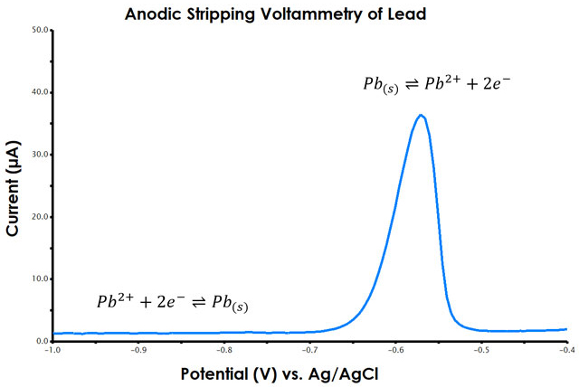
Figure 1. Anodic Stripping Voltammetry (ASV) of Lead

 
First, a water sample is pre-treated to convert any solid lead into its ionic form (Pb2+).  Chelating ligands, such as acetate, are often added to facilitate extraction, dissolution, and stabilization of lead.  Other salts may also be added as ions of supporting electrolyte, or as buffer components for pH control.
 
Second, Pb2+ is converted to Pb and deposited at a mercury (Hg) electrode under a reduction potential as shown in Equation 1.
\displaystyle{Pb^{2+} + 2e^{-}\rightleftharpoons Pb_{(s)}} (1)
 
Bare carbon screen-printed electrode and mercury plated screen-printed electrode

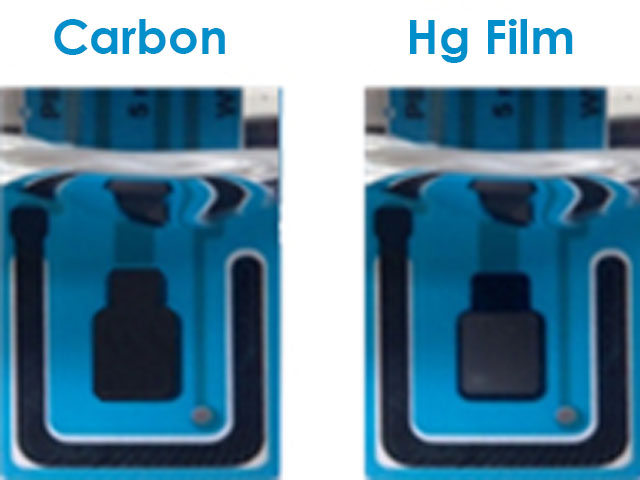
Figure 2. Bare Carbon Screen-Printed Electrode and Mercury-Plated Screen-Printed Electrode

 
There are two types of Hg electrodes commonly used in ASV analysis: hanging mercury drop (HMD) and mercury film (MF).
 
An HMD electrode is formed at the end of a capillary tube that is filled with Hg and the other end of the tube is connected to an Hg reservoir.  HMD electrodes can be regenerated by discarding an old drop and forming a new one.  This desirable characteristic makes it easy to obtain a clean, reproducible Hg surface.  In comparison, the surface of an MF type electrode cannot be regenerated.  However, such an electrode is simple in construction, and consists of many microscopic Hg droplets (μm in diameter) adhering on a carbon substrate surface.
 
The high surface-area-to-volume ratio of the Hg droplets enhances mass transfer rate.  Thus, during the same enrichment time, an MF electrode can electrolyze more Pb into the Hg than at an HMD electrode.
 
Finally, the Pb enriched in Hg is oxidized and converted back to Pb2+ as the electrode potential is swept toward a positive limit (see Equation 2).
\displaystyle{Pb_{(s)} \rightleftharpoons Pb^{2+} + 2e^{-}} (2)
In a very short time (as compared to the time of enrichment), all Pb that was pre-concentrated into the Hg droplets is oxidized to Pb2+ and released back into the electrolyte solution.  The name anodic stripping refers to this step, where Pb is stripped out of Hg via electrochemical oxidation.
 
During anodic stripping, current is recorded while the electrode potential is swept linearly.  If the linear sweep is a pure monotonic ramp, then the technique is called linear sweep voltammetry (LSV). Linear Sweep Voltammetry (LSV) Sometimes, a pulse train is superimposed onto the linear sweep to enhance the sensitivity.  In this lab, we will use such a pulse technique named differential pulse voltammetry (DPV). Differential Pulse Voltammetry (DPV)
Back To Top

4Differential Pulse Voltammetry

Differential Pulse Voltammetry Differential Pulse Voltammetry (DPV) measures the difference in current before and after a potential pulse.  Compared to LSV, this technique avoids measurement of the current due to double layer charging (capacitive current), which contains little information of interest for stripping analysis.  In addition, the time delay (at constant potential) before each pulse allows the depletion zone just adjacent to the electrode surface to recover.  Consequently, a larger peak current is detected in DPV when compared to LSV.
Back To Top

5Solution Preparation

Due to the sensitivity of ASV, all glassware should be soaked in 3M HNO3 for at least 24 hours.
 
  1. Nitric Acid Solution (3.0 M) - Prepare 1 L of 3.0 M nitric acid solution.  For this solution, you will need concentrated nitric acid (HNO3, 68.9%).  CAUTION: Nitric acid is highly corrosive.  Avoid contact with skin.  If any contacts the skin, rinse profusely with copious amounts of water.  Into a 1 L volumetric flask and under constant stirring, slowly add 190 mL of concentrated HNO3 to approximately 700 mL of water.  Dilute to the mark with distilled water.  Label the solution as "3 M HNO3 Solution".  The nitric acid solution is for cleaning all glassware.
  2. Hydrochloric Acid Solution (1.0 M) - Prepare 100 mL of 1.0 M hydrochloric acid solution.  For this solution, you will need high purity, concentrated hydrochloric acid (HCl, 37%).  CAUTION: Hydrochloric acid is highly corrosive.  Avoid contact with skin.  If any contacts the skin, rinse profusely with copious amounts of water.  Add 8.3 mL of concentrated HCl to approximately 70 mL of deionized water.  Mix gently and dilute to the mark with deionized water.  Label this solution as "1 M HCl Solution".
  3. Mercury Acetate (4 mM) in 0.2 M Hydrochloric Acid Solution - Prepare 100 mL of 4.0 mM mercury acetate (Hg(CH3COO)2, MW = 318.7 g/mol) in 0.2 M HCl acid solution.  In a 100 mL volumetric flask, add 20 mL of 1 M HCl solution to approximately 50 mL deionized water.  Dissolve 0.13 g Hg(CH3COO)2 into the solution.  Dilute to the mark with deionized water.  Label this solution as "4 mM Hg(CH3COO)2 in 0.2 M HCl Solution".
  4. Mercury Acetate (0.4 mM) in 20 mM Hydrochloric Acid Solution - Prepare 100 mL of 0.4 mM Hg(CH3COO)2 in 20 mM acid solution by dilution of the 4 mM Hg(CH3COO)2 in 0.2 M HCl solution.  In a 100 mL volumetric flask, add 10 mL of the 4 mM Hg(CH3COO)2 in 0.2 M HCl solution and dilute to the mark with deionized water.  Label this solution as "0.4 mM Hg(CH3COO)2 in 0.2 mM HCl Solution".
  5. Sodium Acetate (NaOAc) Buffer (1.0 M) - Prepare 100 mL of 1.0 M sodium acetate Buffer (Na(CH3COO), MW = 82.03 g/mol).  Sodium acetate is abbreviated NaOAc.  In a 100 mL volumetric flask, dissolve 8.20 g NaOAc in 50 mL deionized water.  Add 4.2 mL of concentrated HCl and dilute to the mark with deionized water.  Label this solution as "1.0 M NaOAc buffer".
  6. Sodium Acetate (NaOAc) Buffer (20 mM) - Prepare 1 L of 20 mM sodium acetate buffer.  Prepare this solution by dilution of the 1.0 M NaOAc buffer previously prepared.  In a 1 L volumetric flask, add 20 mL of the 1.0 M NaOAc buffer to approximately 700 mL deionized water and dilute to the mark.  Label this solution as "20 mM NaOAc Buffer".
  7. 1000 ppm Lead Acetate (1000 ppm) in 20 mM NaOAc Buffer - Prepare 100 mL of 1000 ppm (4.83 mM) lead acetate (Pb(CH3COO)2, MW = 325.29 g/mol) in 20 mM NaOAc buffer.  In a 100 mL volumetric flask, dissolve 0.18 g of Pb(CH3COO)2 in 70 mL of 20 mM NaOAc buffer, then dilute to the mark with 20 mM NaOAc buffer.  Label this solution as "1000 ppm Pb2+in 20 mM NaOAc Buffer".
  8. Lead Acetate (1 ppm) in 20 mM NaOAc Buffer - Prepare 100 mL of 1 ppm (4.83 μM) in 20 mM NaOAc buffer by dilution of the 1000 ppm Pb(CH3COO)2 buffer solution previously prepared.  In a 100 mL volumetric flask, add 100 μL of the 1000 ppm Pb2+ in NaOAc buffer to ~70 mL of the 20 mM NaOAc buffer.  Mix gently then dilute to the mark with 20 mM NaOAc buffer.  Label this solution "1 ppm Pb2+ in 20 mM NaOAc Buffer".
Back To Top

6Setup and Preparation

6.1Physical Setup

For this lab, obtain a stirrer, magnetic stir bar, Pine Research WaveNow potentiostat, 
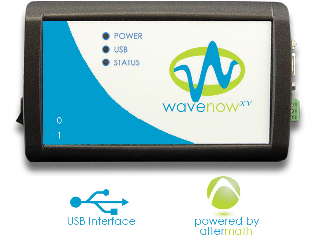
WaveNowXV Potentiostat Bundles compact voltammetry kit, Screen-Printed Electrode Cell Starter Kit large volume compact voltammetry cell (AKSPEJAR), Screen-Printed Electrode Large Volume Cell and 5x4 mm carbon screen-printed electrodes. 
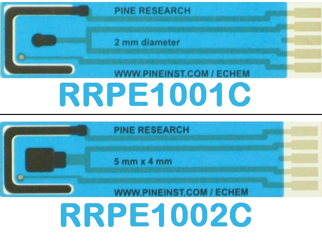
Carbon Screen-Printed Electrodes
 
There are two main components of the electrochemical measurement system used in this experiment: the potentiostat and the electrodes.  Often, three electrodes are used with a potentiostat and are called the working, counter, and reference electrodes.
 
The electrochemical reaction of interest occurs at the working electrode.  The working electrode, in this particular case, is an inert material that functions as a sink for electron transfer.  The reference electrode has its own standard and reversible electrochemical potential and serves as a standard reference for cell potential.  Current should never flow through a reference electrode; thus, the counter electrode (or auxiliary electrode) is the third electrode in the system.  Charge flows (as current) through the counter electrode to balance a change in cell potential, due to the reaction at the working electrode.  For this experiment, the screen-printed electrode contains all three electrodes (see Figure 3).
 
5x4 mm carbon screen-printed electrode

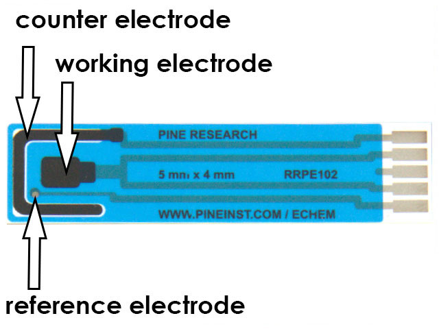
Figure 3. 5x4 mm Carbon Screen-Printed Electrode

Back To Top

6.2Mercury Deposition

The first experimental step in this laboratory is to deposit a layer of mercury microdroplets onto the surface of a carbon working electrode.  Hg is reduced to the working electrode by application of a reductive (negative) potential.  Hg deposition to the carbon electrode need only be done one time for this laboratory.  As long as the Hg layer is not oxidized from the carbon surface, it will remain stable and intact during DPV stripping.
 
Connect a 5x4 mm carbon screen-printed electrode to the compact voltammetry hand grip as shown in Figure 4.  You should have between one to two small spacers inserted into the grip, behind the screen-printed electrode, otherwise the electrode will not stay in place.  The grip and electrode fit into the tan cap, which fits into the large volume compact voltammetry electrochemical cell.
 
Carbon screen-printed electrode connected to grip mount

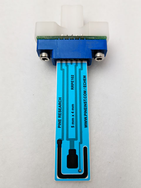
Figure 4. Carbon Screen-Printed Electrode Connected to Grip Mount

 
The tan cell cap has two small holes for purge lines.  Insert one length of the purge tubing into solution, touching the bottom of the cell (called the purge line).  Insert another length of the purge tubing into the cell, but above the solution level (called the blanket line) (see Figure 5).
 
Cell setup for mercury deposition onto carbon electrode

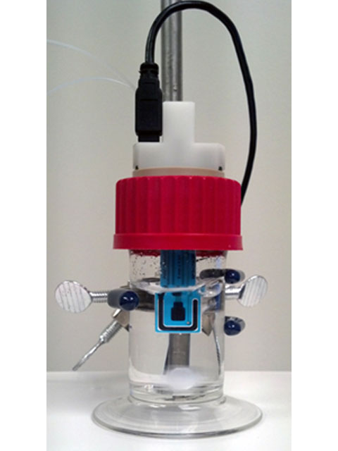
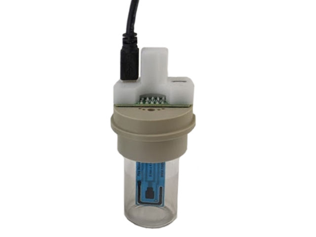
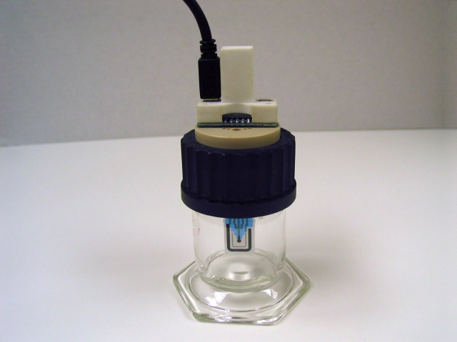
Figure 5. Cell setup for mercury deposition onto carbon electrode

 
Add 15 mL of the 0.4 mM Hg(CH3COO)2 in 0.2 mM HCl solution into the electrochemical cell.  Add a magnetic stir bar to the cell.  Set the constant stir rate appropriate for the cell dimensions, around 500 RPM.  The stirring should be significant but ensure that solution stays in contact with the screen-printed electrode elements at all times while stirring.  Place the cell on a stirrer and connect to the WaveNow potentiostat as shown (see Figure 6).
 
Components for lead detection lab, including compact voltammetry cell, WaveNow potentiostat and stirrer

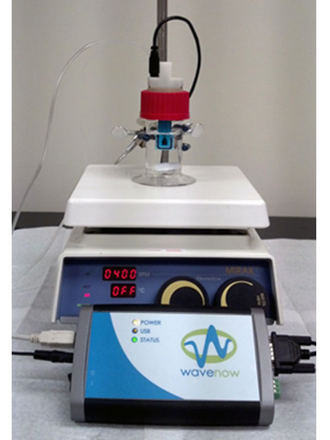
Figure 6. All Components for this Laboratory, Including Compact Voltammetry Cell, Potentiostat and Stirrer

 
Hg microdroplets are formed on the carbon screen-printed electrode surface by reducing Hg2+ to Hg at -1 V vs Ag/AgCl for 15 min in 0.4 mM Hg(CH3COO)2 in 0.2 mM HCl solution.  Within AfterMath, start a new Bulk Electrolysis (BE) Experiment Bulk Electrolysis (BE) (see Figure 7).
 
Bulk electrolysis parameters for mercury deposition in AfterMath

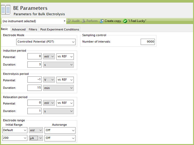
Figure 7. Bulk Electrolysis Parameters for Mercury Deposition in AfterMath

 
Ensure the solution is stirring, then click “Perform” in AfterMath to start the deposition program.  The total time for this part of the experiment can be determined from all steps of the bulk electrolysis and is around 17 minutes.  When the experiment has finished, rinse the electrode thoroughly with deionized water.
 
Store the electrode under N2-sparged water to avoid oxidation of the Hg microdroplets on the electrode surface.
Back To Top

6.3General DPSV Analysis Protocol

The following instructions are a general protocol to perform trace metals determination by DPSV. You should have already completed the previous step to reduce mercury onto the surface of the carbon screen-printed electrode.  The method used in this experiment is called standard addition.
 
  1. Add a stir bar and 50 mL of test solution to the large volume compact voltammetry electrochemical cell.  Insert the screen-printed electrode (plated with Hg) into the hand grip (see Figure 4) and assemble the hand grip and cap into the cell.
  2. Degas the solution by sparging with N2 for at least 10 min.  Turn the three way valve to flow N2 through the purge line.  Continuously bubble N2 through the solution while constantly stirring at a fixed speed (about 500 RPM).  Do not change the stir bar rate for future steps in the experiment.  An easy way to accomplish this is to keep the stirring rate knob fixed in position and simply turn the stirrer off when not in use.
  3. After the solution has been purged for 10 min, the user will complete an anodic stripping voltammetry with DPV experiment (DPSV) (see Figure 8 for suggested DPSV parameters).
  4. The first step in DPSV is to concentrate lead ion into the mercury film (deposition period in AfterMath, also called pre-concentration).  During this step, maintain both stirring and N2 bubbling.  Monitor the experimental progress in AfterMath.  After the deposition period (300 s, as shown in Figure 8), the DPV stripping waveform will start immediately.  Turn off the stirrer and adjust the three way purge valve so N2 enters the cell through the blanket line.  The gas from the blanket line should fill the cell head-space, not agitate solution.  When you discontinue stirring, turn the power off on the stirrer.  DO NOT adjust the RPM knob.
  5. After the experiment has completed, rename or reorganize the DPSV experiment accordingly in AfterMath to indicate the contents of the sample (e.g., 0 ppm Pb2+, pure water).
  6. After measuring the initial sample solution, add an aliquot of 100 μL 1 ppm Pb2+(equivalent to 2 ppb increment in Pb2+ concentration; see Table 1) to the electrochemical cell and repeat steps 4 and 5.  You do not need to repeat the initial purging of solution for 10 minutes, as doing so is only necessary for the initial 50 mL of solution.
  7. Follow the analysis procedure for all solutions listed in Table 1.  Data sufficient for calibration curve construction will be complete when the total added Pb2+ concentration is 10 ppb.
 
Differential Pulse Stripping Voltammetry (DPSV) parameters in AfterMath

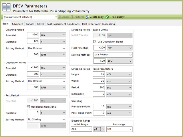
Figure 8. Differential Pulse Stripping Voltammetry (DPSV) Parameters in AfterMath

 
Sample # 1 ppm Pb2+ added to Buffer Standard (µL) Total 1 ppm Pb2+ in Buffer Standard (µL) Known [Pb2+] (ppb)
1 0 0 0
2 100 100 2
3 100 200 4
4 100 300 6
5 100 400 8
6 100 500 10
Table 1. List of Solution Preparation and Composition for Standard Addition
Back To Top

6.4Standard Addition Method

Standard addition is used to minimize any matrix effects.  Matrix effects are unwanted side reactions that can occur simultaneously with the intended reaction and affect the analytical signal of interest.  The species in the matrix can be those that are known as well as unknown.  With standard addition, a series of samples are tested with a constant volume of known standard.  One sample in a series does not contain the standard (or spike).  The analytical signal, DPV peak current, is plotted against concentration.  Standard addition is valid if the agreement between signal and concentration is linear.
 
After a linear regression has been completed across the series of standards and unknown, the line is extrapolated to when current = 0, where the linear regression intersects the x-axis.  The value at this intersection must then be the concentration of the unknown (sign is irrelevant).  In this part of the lab, the user will perform DPSV as before, but with a water sample of unknown Pb2+ concentration.  The goal will be to determine the unknown concentration of Pb2+ in the water sample.
Back To Top

7Experimental

7.1Measurement of Lead in Pure Water by Standard Addition

This laboratory encourages the user to first perform an analysis of pure water with standard additions of Pb2+.  This aids in familiarization of the instrument, utilization of the software, and verification that a linear response can be obtained.
 
For this experiment, the user should place 50 mL of 20 mM NaOAc buffer into the large volume compact voltammetry cell (step 1 in the General DPSV Protocol).  Since an unknown water sample is not used, using entirely buffer solution is appropriate.
 
A total of six solutions will be studied by DPSV (see Table 1).  The first analysis should be completed with sample #1, where Pb2+ is absent.  All Pb2+ additions will be to the same initial volume of buffer.
Back To Top

7.2Unknown Analysis

Here, the user will analyze six unknown water samples (see Table 1).  Water samples will contain some unknown concentration of Pb2+.
 
For this experiment, the user should place 1 mL of 1 M NaOAc buffer and 49 mL of water analyte sample into the large volume compact voltammetry cell (step 1 in the General DPSV Protocol).  Use of the more concentrated buffer solution will maintain appropriate pH conditions but allow the bulk of the test solution to be the unknown water sample.
 
Solutions should be analyzed starting with the lowest concentration of Pb2+.  Subsequent samples should be analyzed in order of increasing Pb2+ concentration.  The first sample does not contain a spike of Pb2+ solution.

INFO: Always analyze solutions with the lower concentration of analyte FIRST.  Then, add aliquots of standard so concentration of analyte is increasing with sample number.

Back To Top

8Data Analysis

After completion of a DPSV experiment by standard addition, the user should have at least six differential pulse voltammograms.  The general analysis includes:
 
  1. Find the DPSV peak height (current) in AfterMath for each sample where Pb2+ was present (five samples for pure water, all six samples for the unknown).  Record the peak current for each sample in a spreadsheet program.
  2. Prepare an overlay plot.  In an overlay plot, all six DPSV voltammograms should be place into a single plot (see Figure 10).
  3. Perform a standard addition linear calibration analysis.  Plot peak current vs. known concentration of Pb2+ as points (see Figure 11).  Perform regression analysis on the data and draw a linear curve of best fit through the data points and record the linear equation of the line.  A correlational coefficient > 0.98 is expected.  Extrapolate the best fit line to the x-axis, where y = 0.
  4. From the slope of the regression, determine the Pb2+ concentration.  This will correspond to the point on the extrapolated regression curve that crosses the x-axis.  This is the concentration of Pb2+ in your unknown sample.
Back To Top

8.1Determine DPSV Peak Height

Determination of a peak height is very easy in Aftermath.  The user can set the appropriate baseline, from which peak height is determined (see Figure 9).  The directions for peak height determination in AfterMath are as follows:
 
  1. In AfterMath, right-click the data trace that contains a peak of interest.
  2. Select "Add Tool", then select "Peak Height".  Three colors or orbs will appear on the plot.  The green orb should be moved onto the peak apex, the highest point in the peak.  You can use the zoom (+ magnifying glass) in Aftermath to fine tune your selection, as well as the scroll wheel if using a mouse.  The pink orbs are the baseline points and the black orbs extend the length of your baseline.
  3. Right-click the pink orb and select properties.  From the menu, choose “free horizontal” as the method by which the baseline is drawn.  Click OK.  Drag and drop the pink orb (notice, a horizontal line is drawn through the pink orb) until the baseline is best drawn through the zero current leading and trailing baseline.
  4. The peak current will be displayed with a line drawn to the green dot.
  5. Record the peak height and known Pb2+ concentration in a spreadsheet program.
 
Differential Pulse Stripping Analysis peak height determination in AfterMath

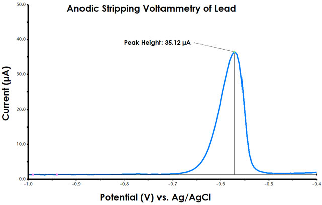
Figure 9. Anodic Stripping Voltammetry Peak Height Determination in AfterMath

Back To Top

8.2Prepare an Overlay Plot

An overlay plot can be made very easily in AfterMath (see examples of overlays in Figure 10).  It is as easy as copying/pasting.  The directions are:
 
  1. Right-click a node in the archive tree structure and select "New", then select "Plot".
  2. For each standard addition, including the first where no standard was added, click the “+” sign next to the DPSV Experiment icon.  Click the “Voltammogram” icon.
  3. Click the data trace (the voltammogram) and copy it (either press Ctrl+C, or select Copy from the edit menu, or right-click the data and select copy).
  4. Click the new plot icon you created in step 1, then click the blank plot in the plot window.  Paste the data (either press Ctrl+V, or select Paste from the edit menu, or right-click the data and select paste).
  5. Repeat steps 2 – 4 for all DPSV obtained in an experiment.  Adjust axes as appropriate.
 
Differential Pulse Stripping Voltammograms for standard addition of Pb2+

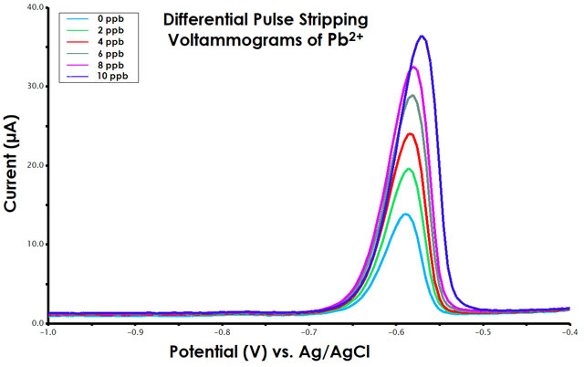
Figure 10. Differential Pulse Stripping Voltammograms for Standard Addition of Pb2+

Back To Top

8.3Construct Standard Addition Plot

In a graphing program of your choice (e.g., Microsoft Excel), create a scatter plot for your data obtained for each experiment (see Figure 11).  The general directions are as follows:
 
  1. Plot peak current (from section 8.1) on the y-axis and known concentration of Pb2+ on the x-axis.
  2. Display the data as points, no connecting line.
  3. Perform regression analysis on the data points; i.e., add a trend line and view the resulting equation and correlational coefficient.  Record the regression (linear) equation.  The correlational coefficient should be > 0.98.
  4. For DPSV in pure water, the intercept will be close to (0,0) since one would not expect current when no Pb2+ was present to strip.  For DPSV of unknown samples, the intercept will not be zero.
  5. Extrapolate the regression line to the x-axis (when y = 0 for the linear equation).
 
Standard addition plot for [Pb2+] in tap water by differential pulse stripping voltammetry

Figure 11. Standard Addition Plot for [Pb2+] in Tap Water by Differential Pulse Stripping Voltammetry

Back To Top

8.4Determine Unknown Lead Concentration

After the standard addition plot has been constructed, simply determine the x-axis intercept of the regression line.  This can easily be done from the equation of the line found during regression analysis.
 
The overlay example shows data for public sewer water obtained in Pennsylvania (see Figure 10).  The standard addition plot (see Figure 11) was based upon the voltammograms shown in the overlay example (see Figure 10).  The linear equation for the regression is shown in Equation 3:
\displaystyle{y = 2.437x + 12.91,  R^{2} = 0.997} (3)
It was determined that the unknown concentration of lead in the public water sampled was 5.30 ppb.  The action limit for lead in water in Pennsylvania is 15 ppb.
Back To Top

9Questions

  1. What is the unknown concentration of lead in the water analyzed?  If drinking water was analyzed, how does the concentration compare to the legal limit in public drinking water?
  2. What is the purpose of purging and blanketing with nitrogen gas?  What might you expect would happen if this step was not performed?
  3. Why is the stir bar used in the pre-concentration step of a differential pulse anodic stripping voltammetry experiment?  What do you expect would be the result if the solution was not stirred during this step?
  4. Write the electrochemical half reaction of interest that occurs during the mercury plating process, the pre-conditioning step, and the stripping step of DPSV.
  5. Stripping voltammetry can detect several metals at the same time, as long as their thermodynamic electrode potentials are separated by about 100 mV.  Draw the stripping voltammogram you would expect for a mixture of Cd2+, Pb2+, and Cu2+ (HINT: look up the appropriate half reactions in a textbook).
Back To Top

10References

Back To Top
Questions? Find Answers.

Our knowledgebase is the central repository for written content, including help topics, theory, application notes, specifications, and software information.

Select a category below or view the Knowledgebase home page
Software

Detailed information about our Software, which includes AfterMath and retired PineChem.

Applications

Application notes discuss practical aspects of conducting specific experiments.

Theory

Fundamental electrochemical theory presented in a brief and targeted manner.

Product Specifications

Review complete product specifications and compare products within a category here.